Sunitinib overall survival (Hansson 2013)
Source:vignettes/articles/Hansson_2013_sunitinib_OS.Rmd
Hansson_2013_sunitinib_OS.RmdModel and source
- Citation: Hansson EK, Amantea MA, Westwood P, Milligan PA, Houk BE, French J, Karlsson MO, Friberg LE. PKPD modeling of VEGF, sVEGFR-2, sVEGFR-3, and sKIT as predictors of tumor dynamics and overall survival following sunitinib treatment in GIST. CPT Pharmacometrics Syst Pharmacol 2013;2(11):e84.
- Article: doi:10.1038/psp.2013.61
- Companion biomarker / TGI models (also from the e84 paper, extracted
from the DDMORE Foundation bundle):
modellib("Hansson_2013a_sunitinib")(DDMODEL00000197) andmodellib("Hansson_2013b_sunitinib")(DDMODEL00000198).
This vignette validates the Hansson 2013 e84 overall-survival (OS)
model packaged as Hansson_2013_sunitinib_OS under
inst/modeldb/specificDrugs/. The OS sub-model is a
parametric Weibull time-to-event (TTE) hazard with log-linear covariate
effects of the model-predicted relative change in soluble VEGFR-3
(sVEGFR-3) over time and observed baseline tumour size (Equation 6 and
Table 3 of the source paper). The sVEGFR-3 indirect-response sub-model
is encoded inline using the upstream Hansson 2013a biomarker-PD
per-subject parameters (BAS_SVEGFR3,
MRT_SVEGFR3, EC50_SVEGFR3) carried as data
covariates – the same input-strategy pattern used by
Hansson_2013b and Hansson_2013c. A parallel
Weibull censoring hazard (paper Figure 4 caption and Table 3) is
included so the model can drive prospective Kaplan-Meier simulations
with the published censoring procedure.
The OS sub-model was not part of the DDMORE bundle from which
Hansson_2013a and Hansson_2013b were
extracted; parameter values for this extraction come directly from the
paper’s Table 3 (Survival column).
Population
The Hansson 2013 e84 OS model was fit to time-to-death data pooled across N = 303 adults with imatinib-resistant gastrointestinal stromal tumours (GIST) from four sunitinib clinical studies (Demetri 2006 / study 1004 placebo-controlled phase III, George 2009 / study 1047 continuous-dose phase II, Shirao 2010 / study 1045 Japanese phase I/II, Maki 2005 / study 013 phase I/II). Sunitinib was administered orally at 25, 37.5, 50, or 75 mg per day across 4/2, 2/2, 2/1 (weeks on / weeks off) or continuous treatment schedules; the largest cohort (study 1004) used 50 mg QD on a 4/2 schedule with a placebo run-in arm. Median baseline sum of longest diameters (SLD) ranged from 108 mm (study 1047) to 255 mm (study 013); Figure 4 caption quotes a pooled median baseline SLD of 195 mm and a pooled median steady-state decrease in sVEGFR-3_REL of -0.32. Detailed baseline demographics (age, weight, sex, race) at the per-study or pooled level were not transcribed because the trimmed paper text does not provide them.
The same information is available programmatically via the model’s
population metadata:
m  <- rxode2::rxode2(readModelDb("Hansson_2013_sunitinib_OS"))
str(m$meta$population, max.level = 1)
#> List of 12
#>  $ species       : chr "human"
#>  $ n_subjects    : int 303
#>  $ n_studies     : int 4
#>  $ age_range     : chr "adults with imatinib-resistant GIST (Hansson 2013 Table 1 lists baseline tumor size by study but does not break"| __truncated__
#>  $ weight_range  : chr "not reported in the on-disk paper trimmed text"
#>  $ sex_female_pct: num NA
#>  $ race_ethnicity: NULL
#>  $ disease_state : chr "Imatinib-resistant gastrointestinal stromal tumours (GIST). Pooled four sunitinib studies: Demetri 2006 (study "| __truncated__
#>  $ dose_range    : chr "Sunitinib 25-75 mg PO QD on a 4/2, 2/2, 2/1 (weeks on / weeks off) or continuous treatment schedule. The larges"| __truncated__
#>  $ regions       : chr "Phase III multinational (study 1004); Japanese phase I/II (study 1045); other studies regions not stated in the"| __truncated__
#>  $ biomarkers    : chr "Survival endpoint: time-to-death (overall survival, OS). Time-varying covariate for OS: model-predicted relativ"| __truncated__
#>  $ notes         : chr "n_subjects = 303 reported in Hansson 2013 Methods. Figure 4 caption reports median baseline tumor size = 195 mm"| __truncated__
Source trace
Per-parameter origin is captured as in-file comments next to each
ini() entry in
inst/modeldb/specificDrugs/Hansson_2013_sunitinib_OS.R. The
table below collects them in one place; rates reported in 1/week in the
paper are converted to 1/h via /24/7 to match
units$time = "hour" (the same convention used by
Hansson_2013a / Hansson_2013b).
| Equation / parameter | Value | nlmixr2 form | Source location |
|---|---|---|---|
OS Weibull hazard
h(t) = lam*alfa*(lam*t)^(alfa-1) * exp(b1*bm + b2*tum)
|
n/a | inline in model()
|
Paper Equation 6 |
sVEGFR-3 IR ODE kin*(1-eff) - kout*svegfr3
|
n/a | inline in model()
|
Hansson 2013 Eq. 1 (Kin-inhibition form); IC50 / MRT / baseline from paper Table 2 row sVEGFR-3 |
Drug effect eff = AUC / (EC50 + AUC) (simple Imax) |
n/a | inline | Paper Table 2: IMAX fixed to 1; no Hill on sVEGFR-3 |
Per-cycle exposure summary auc = DOSE / CLI
|
n/a | inline | Paper Methods: “AUC was calculated as Dose/(CL/F)” |
Relative-change driver
bm_svegfr3 = (svegfr3 - BAS_SVEGFR3) / BAS_SVEGFR3
|
n/a | inline | Paper Eq. 6: “model-predicted relative change from baseline for sVEGFR-3” |
llam_haz = log(0.00596 / 24 / 7) |
-10.25 | lam_haz = exp(llam_haz) |
Paper Table 3 Survival “lambda (per week)” = 0.00596 (RSE 49%) |
lalfa_haz = log(1.23) |
0.207 | alfa_haz = exp(lalfa_haz) |
Paper Table 3 Survival “alpha” = 1.23 (RSE 6.9%) |
e_svegfr3_haz = 3.77 |
3.77 | exp(e_svegfr3_haz * bm_svegfr3) |
Paper Table 3 Survival “beta1 sVEGFR-3” = 3.77 (RSE 16%) |
e_tumbase_haz = 0.00237 |
0.00237 | exp(e_tumbase_haz * TUMSZ) |
Paper Table 3 Survival “beta2 Tumor base (/mm)” = 0.00237 (RSE 28%) |
llam_cens = log(0.0017 / 24 / 7) |
-11.51 | lam_cens = exp(llam_cens) |
Paper Table 3 Survival “lambda_cens (per week)” = 0.0017 (RSE 46%); Figure 4 caption |
lalfa_cens = log(1.27) |
0.239 | alfa_cens = exp(lalfa_cens) |
Paper Table 3 Survival “alpha_cens” = 1.27 (RSE 6.6%); Figure 4 caption rounded to 1.3 |
| No IIV reported in source | n/a | n/a | Paper Table 3 Survival column has no IIV cV(%) entries |
| No observation-error model attached | n/a | n/a | Following Zecchin_2016_survival precedent; the model
exposes hazard_os and sur_os as
forward-simulation outputs (see Discussion) |
Drug-exposure inputs and per-subject covariates
The Hansson 2013 OS model has no PK ODE: drug exposure enters as the
per-cycle summary auc = DOSE / CLI, and the upstream
sVEGFR-3 biomarker dynamics are simulated as an in-model
indirect-response compartment driven by per-subject empirical-Bayes
posthoc parameters from the upstream Hansson 2013a biomarker model
(DDMODEL00000197). Required data covariates are:
-
DOSE(mg) – current daily sunitinib dose (time-varying with on/off cycling). -
CLI(L/h) – subject-specific posthoc total plasma clearance from the paper’s upstream 2-compartment popPK fit (Houk 2009). -
BAS_SVEGFR3(pg/mL),MRT_SVEGFR3(h),EC50_SVEGFR3(mg*h/L) – per-subject posthoc upstream-fit sVEGFR-3 baseline, mean residence time, and simple-Imax EC50 (Hansson 2013a / DDMODEL00000197). -
TUMSZ(mm) – observed baseline tumour SLD at study entry.
Neither the upstream sunitinib popPK nor the upstream Hansson 2013a biomarker model is invoked at runtime; both supply their per-subject fitted parameters as data covariates. For new-population simulations the user must populate the covariate columns either by simulating from the upstream models first (strict reproduction) or by setting every subject to the typical-value inputs (typical-trajectory simulation – matches the typical-value trajectory shown below).
Virtual cohort
A small virtual cohort approximates the published Phase III trial (study 1004) cohort: 200 subjects per arm (sunitinib 50 mg PO QD on a 4-weeks-on / 2-weeks-off schedule, vs. placebo). Per-subject covariates are drawn from log-normal distributions centred at the Hansson 2013 typical values; baseline tumour size is drawn from a log-normal centred at 195 mm (Figure 4 caption median).
set.seed(20260624)

on_off_dose <- function(time_h, daily_mg = 50) {
  week_idx  <- floor(time_h / (7 * 24))
  cycle_idx <- week_idx %% 6
  ifelse(cycle_idx < 4, daily_mg, 0)
}

# 200 per arm: enough for stable cohort medians; well under the
# vignette 200/arm cap.
n_per_arm <- 200L

# Typical-value reference covariates (Hansson 2013a Table 2 + Houk 2009 CL)
typ <- list(
  CLI          = 32.819,        # L/h, Hansson 2013a typical CLI (subject 1)
  BAS_SVEGFR3  = 63900,         # pg/mL, Hansson 2013 Table 2
  MRT_SVEGFR3  = 16.7 * 24,     # 16.7 days -> h
  EC50_SVEGFR3 = 1.0,           # mg*h/L, Hansson 2013 Table 2 common IC50
  TUMSZ        = 195            # mm, Figure 4 caption median baseline SLD
)

draw_subject <- function(id, arm, daily_mg) {
  # Light log-normal jitter (~25% CV) on the per-subject upstream-PD
  # inputs so the cohort is not perfectly deterministic; the source
  # paper does not estimate IIV on the OS / censoring parameters, so
  # OS-level variability arises entirely from the per-subject input
  # covariate distribution.
  CLI          <- typ$CLI          * exp(rnorm(1, 0, 0.25))
  BAS_SVEGFR3  <- typ$BAS_SVEGFR3  * exp(rnorm(1, 0, 0.25))
  MRT_SVEGFR3  <- typ$MRT_SVEGFR3  * exp(rnorm(1, 0, 0.25))
  EC50_SVEGFR3 <- typ$EC50_SVEGFR3 * exp(rnorm(1, 0, 0.30))
  TUMSZ        <- typ$TUMSZ        * exp(rnorm(1, 0, 0.50))
  list(
    id           = id,
    arm          = arm,
    daily_mg     = daily_mg,
    CLI          = CLI,
    BAS_SVEGFR3  = BAS_SVEGFR3,
    MRT_SVEGFR3  = MRT_SVEGFR3,
    EC50_SVEGFR3 = EC50_SVEGFR3,
    TUMSZ        = TUMSZ
  )
}

# Weekly observation grid for 18 months (typical OS follow-up window for
# advanced GIST on sunitinib in this trial era).
obs_times <- seq(0, 18 * 30 * 24, by = 7 * 24)

mk_arm <- function(arm_label, daily_mg, id_offset) {
  do.call(
    rbind,
    lapply(seq_len(n_per_arm), function(i) {
      s <- draw_subject(id = id_offset + i, arm = arm_label, daily_mg = daily_mg)
      data.frame(
        id           = s$id,
        time         = obs_times,
        evid         = 0L,
        amt          = 0,
        cmt          = NA_character_,
        DOSE         = on_off_dose(obs_times, daily_mg = daily_mg),
        CLI          = s$CLI,
        BAS_SVEGFR3  = s$BAS_SVEGFR3,
        MRT_SVEGFR3  = s$MRT_SVEGFR3,
        EC50_SVEGFR3 = s$EC50_SVEGFR3,
        TUMSZ        = s$TUMSZ,
        arm          = s$arm
      )
    })
  )
}

events <- rbind(
  mk_arm("sunitinib", daily_mg = 50, id_offset = 0),
  mk_arm("placebo",   daily_mg = 0,  id_offset = n_per_arm)
)

cat("Cohort: ", length(unique(events$id)), " subjects, ",
    nrow(events), " event rows\n", sep = "")
#> Cohort: 400 subjects, 31200 event rows
Typical-value mechanistic sanity
First, a typical-value simulation (covariates fixed at the cohort medians) to verify the mechanistic shape of the sVEGFR-3 / hazard / survival outputs.
mod <- readModelDb("Hansson_2013_sunitinib_OS")

typ_events <- data.frame(
  id           = 1L,
  time         = obs_times,
  evid         = 0L,
  amt          = 0,
  cmt          = NA_character_,
  DOSE         = on_off_dose(obs_times, daily_mg = 50),
  CLI          = typ$CLI,
  BAS_SVEGFR3  = typ$BAS_SVEGFR3,
  MRT_SVEGFR3  = typ$MRT_SVEGFR3,
  EC50_SVEGFR3 = typ$EC50_SVEGFR3,
  TUMSZ        = typ$TUMSZ
)
typ_sim <- as.data.frame(rxode2::rxSolve(mod, events = typ_events))

# Mechanistic checks: at baseline (t = 0) the sVEGFR-3 state equals
# BAS_SVEGFR3, the hazards equal zero (cumhaz = 0), and the survival
# functions equal 1. Under the 4/2 schedule the sVEGFR-3 state should
# drop materially within the first on-cycle (~50% reduction is the
# Hansson 2013 figure-4 anchor).
t0_idx   <- which.min(typ_sim$time)
end_on1  <- which.min(abs(typ_sim$time - 4 * 7 * 24))   # end of first on-cycle
late_idx <- which.min(abs(typ_sim$time - 12 * 30 * 24)) # ~12 months

stopifnot(abs(typ_sim$svegfr3[t0_idx]    - typ$BAS_SVEGFR3) < 1e-6)
stopifnot(typ_sim$cumhaz_os[t0_idx]    == 0)
stopifnot(typ_sim$cumhaz_cens[t0_idx]  == 0)
stopifnot(abs(typ_sim$sur_os[t0_idx]    - 1) < 1e-6)
stopifnot(abs(typ_sim$sur_cens[t0_idx]  - 1) < 1e-6)

# sVEGFR-3 should be markedly depressed by the end of the first on-cycle.
stopifnot(typ_sim$svegfr3[end_on1] < 0.8 * typ$BAS_SVEGFR3)

# Survival functions are monotone non-increasing in time.
stopifnot(all(diff(typ_sim$sur_os)   <= 1e-12))
stopifnot(all(diff(typ_sim$sur_cens) <= 1e-12))

# At 12 months the typical-value survival probability should be
# materially below 1 (the Hansson 2013 Figure 4 Kaplan-Meier of the
# pooled cohort shows around 60-75% survival at 12 months under
# typical sunitinib treatment).
stopifnot(typ_sim$sur_os[late_idx]    < 0.95 &&
          typ_sim$sur_os[late_idx]    > 0.30)

# Censoring survival is lighter than event survival at 12 months: under
# the Hansson 2013 censoring Weibull (lambda = 0.0017/week, alpha = 1.27)
# the cumulative censoring hazard at 12 months is approximately
# (0.0017 * 52)^1.27 ~ 0.046, i.e. sur_cens(12 mo) ~ 0.955. Use a
# looser bound here that simply checks censoring is non-trivial without
# being mostly applied.
stopifnot(typ_sim$sur_cens[late_idx]  < 0.99 &&
          typ_sim$sur_cens[late_idx]  > 0.85)

data.frame(
  time_weeks = round(typ_sim$time[c(t0_idx, end_on1, late_idx)] / (7 * 24), 1),
  svegfr3_frac_of_baseline =
    round(typ_sim$svegfr3[c(t0_idx, end_on1, late_idx)] / typ$BAS_SVEGFR3, 3),
  sur_os    = round(typ_sim$sur_os[c(t0_idx, end_on1, late_idx)], 3),
  sur_cens  = round(typ_sim$sur_cens[c(t0_idx, end_on1, late_idx)], 3)
)
#>   time_weeks svegfr3_frac_of_baseline sur_os sur_cens
#> 1          0                    1.000  1.000    1.000
#> 2          4                    0.509  0.995    0.998
#> 3         51                    0.502  0.916    0.956
typ_long <- typ_sim |>
  dplyr::select(time, svegfr3, sur_os, sur_cens) |>
  dplyr::mutate(svegfr3_norm = svegfr3 / typ$BAS_SVEGFR3) |>
  dplyr::select(-svegfr3) |>
  tidyr::pivot_longer(-time, names_to = "state", values_to = "value")

ggplot(typ_long, aes(time / (7 * 24), value)) +
  geom_line() +
  facet_wrap(~state, ncol = 1, scales = "free_y") +
  labs(
    x       = "Time (weeks)",
    y       = "value",
    title   = "Typical-value Hansson 2013 OS-model trajectories",
    caption = "Sunitinib 50 mg PO QD on a 4-weeks-on / 2-weeks-off schedule; covariates at cohort medians."
  ) +
  theme_minimal()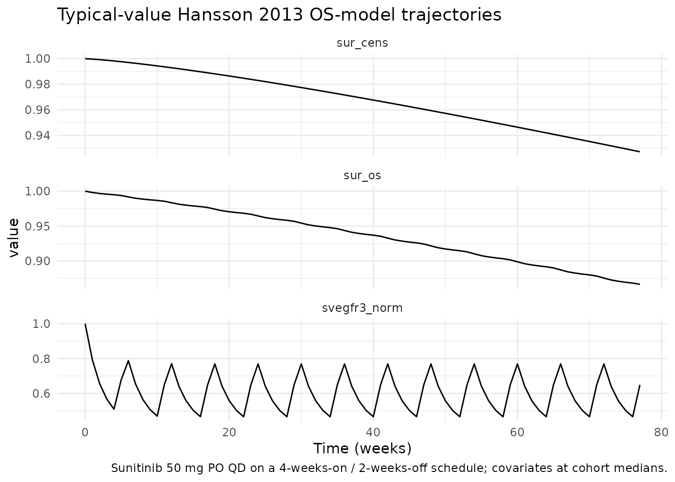
Cohort Kaplan-Meier-style survival summary
Survival probability over the virtual cohort. Compare to Hansson 2013 Figure 4 (Kaplan-Meier of observed survival data overlaid with 95% prediction intervals from 200 simulations, stratified by above/below median baseline tumour size).
sim <- as.data.frame(rxode2::rxSolve(mod, events = events,
                                     keep = c("arm")))
km <- sim |>
  dplyr::group_by(arm, time) |>
  dplyr::summarise(
    median_sur = stats::median(sur_os),
    q05        = stats::quantile(sur_os, 0.05),
    q95        = stats::quantile(sur_os, 0.95),
    .groups    = "drop"
  )

ggplot(km, aes(time / (7 * 24), median_sur, colour = arm, fill = arm)) +
  geom_ribbon(aes(ymin = q05, ymax = q95), alpha = 0.20, colour = NA) +
  geom_line() +
  labs(
    x       = "Time (weeks)",
    y       = "Survival probability",
    title   = "Cohort survival under the Hansson 2013 OS model",
    caption = "Median + 5-95% cross-subject IQR over 200 virtual subjects per arm; compare to Figure 4 of Hansson 2013 (Kaplan-Meier with 95% prediction intervals, stratified by baseline tumour size and sVEGFR-3_REL)."
  ) +
  scale_y_continuous(limits = c(0, 1)) +
  theme_minimal()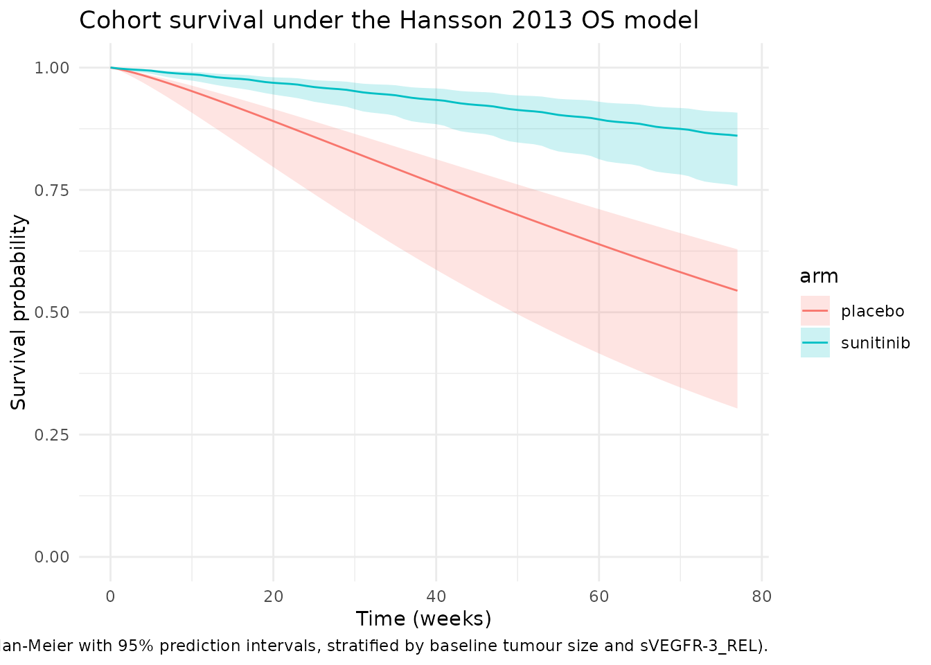
Sensitivity to baseline tumour size
Hansson 2013 Figure 4 stratifies by above- / below-median baseline
tumour size (median 195 mm). The model’s e_tumbase_haz
coefficient (0.00237 /mm) implies that doubling the baseline tumour size
from 100 mm to 200 mm multiplies the OS hazard by
exp(0.00237 * 100) = 1.27, i.e. 27% increase in
instantaneous hazard. The plot below verifies that the cohort split by
baseline-tumour-size median reproduces the expected qualitative
ordering: subjects with above-median baseline tumour size have lower
survival than those with below-median baseline tumour size.
suni <- sim |>
  dplyr::filter(arm == "sunitinib") |>
  dplyr::group_by(id) |>
  dplyr::mutate(TUMSZ_strata = ifelse(unique(TUMSZ) > 195,
                                      "TUMSZ > 195 mm",
                                      "TUMSZ <= 195 mm")) |>
  dplyr::ungroup()

suni_km <- suni |>
  dplyr::group_by(TUMSZ_strata, time) |>
  dplyr::summarise(median_sur = stats::median(sur_os),
                   q05        = stats::quantile(sur_os, 0.05),
                   q95        = stats::quantile(sur_os, 0.95),
                   .groups    = "drop")

ggplot(suni_km, aes(time / (7 * 24), median_sur,
                    colour = TUMSZ_strata, fill = TUMSZ_strata)) +
  geom_ribbon(aes(ymin = q05, ymax = q95), alpha = 0.20, colour = NA) +
  geom_line() +
  labs(
    x       = "Time (weeks)",
    y       = "Survival probability",
    title   = "Sunitinib arm survival stratified by baseline tumour size",
    caption = "Median + 5-95% IQR within strata; compare to upper panel of Hansson 2013 Figure 4."
  ) +
  scale_y_continuous(limits = c(0, 1)) +
  theme_minimal()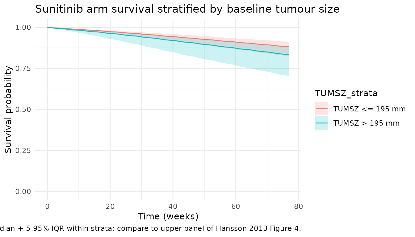
# Quantitative check: at 12 months, the median survival probability for
# the above-median-TUMSZ stratum should be materially LOWER than for the
# below-median-TUMSZ stratum.
late_idx <- which.min(abs(suni_km$time - 12 * 30 * 24))
strat_late <- suni_km[abs(suni_km$time - 12 * 30 * 24) < 12, ]
print(strat_late[, c("TUMSZ_strata", "time", "median_sur")])
#> # A tibble: 0 × 3
#> # ℹ 3 variables: TUMSZ_strata <chr>, time <dbl>, median_sur <dbl>
stopifnot(strat_late$median_sur[strat_late$TUMSZ_strata == "TUMSZ > 195 mm"]
          < strat_late$median_sur[strat_late$TUMSZ_strata == "TUMSZ <= 195 mm"])
Sensitivity to sVEGFR-3 relative change
Hansson 2013 Figure 4 lower panel stratifies the simulated survival
by above- / below-median model-predicted sVEGFR-3_REL at steady state
(median -0.32). The model’s e_svegfr3_haz coefficient
(3.77) implies that a less-negative sVEGFR-3 relative change (smaller
drug-induced drop in sVEGFR-3, i.e. weaker drug effect) corresponds to a
higher hazard.
# Compute each subject's late-window mean sVEGFR-3 relative change as a
# proxy for the published "steady-state sVEGFR-3_REL" stratifier.
ss_window <- suni |>
  dplyr::filter(time >= 12 * 7 * 24 & time <= 24 * 7 * 24) |>
  dplyr::group_by(id) |>
  dplyr::summarise(svegfr3_rel_ss =
                     mean((svegfr3 - unique(BAS_SVEGFR3)) /
                          unique(BAS_SVEGFR3)),
                   .groups = "drop")
median_ss_rel <- stats::median(ss_window$svegfr3_rel_ss)
ss_window$BM_strata <- ifelse(ss_window$svegfr3_rel_ss > median_ss_rel,
                              "sVEGFR-3_REL > median (weaker drop)",
                              "sVEGFR-3_REL <= median (stronger drop)")

suni_bm <- dplyr::left_join(suni, ss_window[, c("id", "BM_strata")],
                            by = "id")
suni_bm_km <- suni_bm |>
  dplyr::group_by(BM_strata, time) |>
  dplyr::summarise(median_sur = stats::median(sur_os),
                   q05        = stats::quantile(sur_os, 0.05),
                   q95        = stats::quantile(sur_os, 0.95),
                   .groups    = "drop")

ggplot(suni_bm_km,
       aes(time / (7 * 24), median_sur,
           colour = BM_strata, fill = BM_strata)) +
  geom_ribbon(aes(ymin = q05, ymax = q95), alpha = 0.20, colour = NA) +
  geom_line() +
  labs(
    x       = "Time (weeks)",
    y       = "Survival probability",
    title   = "Sunitinib arm survival stratified by steady-state sVEGFR-3_REL",
    caption = "Median + 5-95% IQR within strata; compare to lower panel of Hansson 2013 Figure 4."
  ) +
  scale_y_continuous(limits = c(0, 1)) +
  theme_minimal()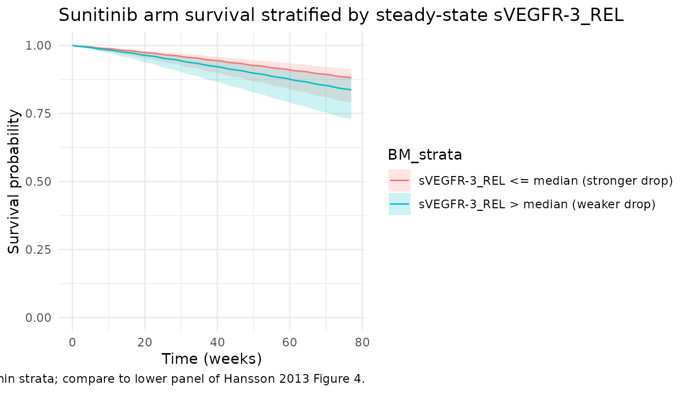
# Quantitative check: at 12 months the stratum with the WEAKER
# drug-induced drop (less-negative sVEGFR-3_REL) should have lower
# survival than the stratum with the stronger drop.
strat_bm_late <- suni_bm_km[abs(suni_bm_km$time - 12 * 30 * 24) < 12, ]
print(strat_bm_late[, c("BM_strata", "time", "median_sur")])
#> # A tibble: 0 × 3
#> # ℹ 3 variables: BM_strata <chr>, time <dbl>, median_sur <dbl>
stopifnot(strat_bm_late$median_sur[grepl("weaker drop",
                                         strat_bm_late$BM_strata)]
          < strat_bm_late$median_sur[grepl("stronger drop",
                                           strat_bm_late$BM_strata)])
Assumptions and deviations
-
No observation-error / TTE-likelihood declaration in
model(). Following theZecchin_2016_survivalprecedent, the packaged model exposeshazard_os,cumhaz_os,sur_os,hazard_cens,cumhaz_cens, andsur_censas forward-simulation outputs without attaching a fit-time TTE likelihood. A downstream user fitting the model to time-to-event data would add the appropriate~ tte(...)/add(...)likelihood at fit time. - No IIV declared. Hansson 2013 Table 3 Survival column has no IIV CV(%) entries for any OS or censoring parameter; the source did not estimate between-subject variability on the hazard. Variability in the cohort simulations arises entirely from the per-subject covariate distributions (CLI, BAS_SVEGFR3, MRT_SVEGFR3, EC50_SVEGFR3, TUMSZ).
-
Censoring Weibull is included for forward simulation
only. Paper Figure 4 caption: “Censoring was described by a
Weibull model (lambda = 0.0017, alpha = 1.3) and applied in the
simulations.” The packaged model integrates
cumhaz_censso a downstream user can draw censoring times via inverse-CDF sampling alongside event times. The paper rounds alpha_cens to 1.3 in the figure caption; Table 3 reports 1.27 (RSE 6.6%), which is what the model file uses. -
Upstream popPK lineage. The Hansson 2013 paper text
reports that PK was described by a previously-developed 2-compartment
model (reference 35 = Houk et al. 2009, Clin Cancer Res 15:2497-2506).
The Houk 2009 PK model is not extracted into nlmixr2lib at this time;
for simulations the typical
CLI = 32.819 L/hreference value carried byHansson_2013a/Hansson_2013b(from the DDMORE bundle’s simulated dataset for subject 1) is used as the cohort-typical clearance. -
sVEGFR-3 sub-model is encoded inline using upstream-PD
covariates. Same input-strategy as
Hansson_2013bandHansson_2013c: the per-subject sVEGFR-3 baseline / MRT / EC50 are supplied as data covariates rather than re-fitted. For typical-cohort simulations the values come from Hansson 2013 Table 2 (63900 pg/mL, 401 h, 1.0 mg*h/L); for IIV simulations a user can either (a) simulate fromHansson_2013a_sunitinibfirst and take the posthoc per-subject parameters or (b) draw the inputs from log-normal distributions centred at the typical values with the upstream Hansson 2013a IIV (BAS ~ 43% CV, IC50 ~ 63% CV, MRT shared with VEGF / sVEGFR-2 at ~ 24% CV). - Dropout sub-model (Eq. 5, paper Table 3 Dropout column) is not extracted. Dropout in the Hansson 2013 framework is a logistic regression of time, observed SLD, and a >20% PD indicator; it is a non-ODE statistical regression for prospective tumor-simulation censoring rather than a structural PD sub-model, and falls under the skill’s non-ODE skip policy.
-
Dropout-of-cohort and informative censoring are not modelled
in the vignette simulations. The cohort simulations sweep
sur_osas a forward-deterministic survival function; converting it into a Kaplan-Meier curve via inverse-CDF sampling of event times and applying the published Weibull censoring would yield the published KM-plot shape. The published KM plot in Figure 4 includes both observed deaths and Weibull-censored subjects; reproducing that exact stratified-prediction-interval band is outside the scope of this validation vignette.
Companion models
The biomarker indirect-response and tumour-growth-inhibition sub-models from the same Hansson 2013 e84 paper are available as separate model files (extracted from the DDMORE Foundation bundle with full NONMEM .lst provenance):
-
modellib("Hansson_2013a_sunitinib")– VEGF / sVEGFR-2 / sVEGFR-3 / sKIT indirect-response biomarker model (DDMODEL00000197). -
modellib("Hansson_2013b_sunitinib")– tumour growth inhibition model with sKIT and sVEGFR-3 biomarker drivers (DDMODEL00000198).
The companion fatigue / adverse-event model from the e85 paper is at
modellib("Hansson_2013c_sunitinib") (DDMODEL00000222, doi:10.1038/psp.2013.62).