Buil-Bruna_2015_lanreotide
Source:vignettes/articles/Buil-Bruna_2015_lanreotide.Rmd
Buil-Bruna_2015_lanreotide.Rmd
library(nlmixr2lib)
library(rxode2)
#> rxode2 5.1.2 using 2 threads (see ?getRxThreads)
#>   no cache: create with `rxCreateCache()`
library(dplyr)
#>
#> Attaching package: 'dplyr'
#> The following objects are masked from 'package:stats':
#>
#>     filter, lag
#> The following objects are masked from 'package:base':
#>
#>     intersect, setdiff, setequal, union
library(tidyr)
library(ggplot2)
library(PKNCA)
#>
#> Attaching package: 'PKNCA'
#> The following object is masked from 'package:stats':
#>
#>     filter
Model and source
- Citation: Buil-Bruna N, Garrido MJ, Dehez M, Manon A, Nguyen TXQ, Gomez-Panzani EL, Troconiz IF. Population Pharmacokinetic Analysis of Lanreotide Autogel/Depot in the Treatment of Neuroendocrine Tumors: Pooled Analysis of Four Clinical Trials. Clin Pharmacokinet. 2016;55(4):461-473. doi:10.1007/s40262-015-0329-4
- Description: One-compartment population PK model with parallel first- and zero-order subcutaneous absorption for lanreotide Autogel/Depot in patients with gastroenteropancreatic neuroendocrine tumors (Buil-Bruna 2015). A linear effect of body weight on apparent clearance and a small categorical effect of sex on the first-order absorbed fraction are retained; absolute bioavailability F is not identifiable and is structurally anchored at 1, so apparent CL/F and Vd/F are reported. Concentrations are predicted in ng/mL; residual error is additive on the log-transformed observations (LTBS), mapped to proportional in linear space.
- Article: Clin Pharmacokinet 55(4):461-473
Lanreotide Autogel/Depot population PK simulation (Buil-Bruna 2015)
Buil-Bruna et al. 2015 pooled four clinical trials (CLARINET, ELECT,
a Spanish multicentre study, and a dose-titration study; 290 patients,
1541 serum samples) to develop a one-compartment population PK model for
lanreotide Autogel/Depot administered every 4 weeks by deep subcutaneous
injection in patients with gastroenteropancreatic neuroendocrine tumors
(GEP-NETs). Absorption is modeled as two parallel mechanisms: a
first-order pathway (rate constant ka, absorbed fraction
F1) responsible for the long apparent terminal half-life
(43.6 days, flip-flop kinetics) and a small zero-order pathway (duration
D0 = 2.96 days, fraction F2 = 1 - F1) that
contributes the early-time concentration peak. The only retained
covariates are a linear effect of body weight on apparent clearance and
a small categorical effect of sex on the first-order absorbed
fraction.
Population
From Buil-Bruna 2015 Table 1 and Methods (Sect. 2.1, 2.3): the pooled dataset is 290 patients with functioning or non-functioning GEP-NETs. Pooled mean age 60.7 years (CV 18.2%; per-study means 58.5-63.3); pooled mean body weight 75.1 kg (CV 22.2%; per-study means 69.3-78.0 kg; population median 74 kg used as the BW covariate reference). Predominantly White patients (race not tested as a covariate); 10 Asian and 10 Black/African American patients (Fig. 5b) provided a retrospective ethnicity sanity check. Renal function spans normal (>90 mL/min, n = 130), mild (60-89, n = 100), moderate (30-59, n = 58), and severe (<30, n = 2). Lanreotide was administered at 60, 90, or 120 mg every 4 weeks; CLARINET, ELECT, and Study 3 were 120 mg only, while Study 4 dose-titrated between 60, 90, and 120 mg. Serum lanreotide was quantified by validated radioimmunoassay (LLOQ 0.078 ng/mL).
The same information is available programmatically as
readModelDb("Buil-Bruna_2015_lanreotide")$population.
Source trace
The per-parameter origin is recorded as an in-file comment next to
each ini() entry in
inst/modeldb/specificDrugs/Buil-Bruna_2015_lanreotide.R.
The table below collects them in one place for review.
| Element | Source location | Value / form |
|---|---|---|
| Structural model | Fig. 2 + Methods Sect. 2.4.2; Results Sect. 3.3.1 | One-compartment disposition; parallel first-order (ka) + zero-order (D0) SC absorption |
| Apparent clearance CL/F | Table 2; Conclusions | 513 L/day at WT = 74 kg |
| Apparent volume Vd/F | Table 2; Abstract | 18.3 L |
| First-order absorption rate ka | Table 2 | 1.59e-2 /day (absorption half-life 43.6 day) |
| First-order absorbed fraction F1 | Table 2; Eq. 1 | 0.994 (female reference) |
| Sex effect on F1 | Table 2; Eq. 1 | -0.024 multiplied by the male indicator (1 - SEXF) |
| Zero-order duration D0 | Table 2 | 2.96 day |
| Body-weight effect on CL/F | Table 2; Eq. 2 | linear: CL/F = theta_CL * [1 + 9.77e-3 * (BW - 74)] |
| Median BW reference | Sect. 3.3.3 | 74 kg |
| IPV CL/F | Table 2 | 27% CV (variance log(1 + 0.27^2) = 0.07031) |
| IPV Vd/F | Table 2 | 150% CV (variance log(1 + 1.50^2) = 1.17865) |
| IPV ka | Table 2 | 61% CV (variance log(1 + 0.61^2) = 0.31641) |
| IPV F1 | Table 2 | 1.05% CV (variance log(1 + 0.0105^2) = 0.0001103) |
| Residual error (LTBS) | Table 2; Methods Sect. 2.4 | sigma_log = 0.275 in log(ng/mL); maps to proportional in linear-space nlmixr2 |
| Bioavailability F (absolute) | Fig. 2 caption | Not identifiable; structurally anchored at 1 (F1 + F2 = 1) |
Virtual cohort
Individual subject-level demographics were not published. We build a virtual cohort of 300 subjects (close to the 290-patient pooled dataset) whose covariate marginals match Buil-Bruna 2015 Table 1: weight log-normal with geometric mean 74 kg and CV ~22%, balanced sex (no sex breakdown is tabulated in the paper but the pooled cohort is clearly mixed). Each subject receives 120 mg lanreotide Autogel/Depot every 4 weeks for 13 doses (about one year of treatment, matching Fig. 4 of the source paper).
set.seed(2015)

n_subj <- 300L

pop <- tibble(
  id     = seq_len(n_subj),
  SEXF   = rbinom(n_subj, size = 1, prob = 0.5),
  WT     = exp(rnorm(n_subj, mean = log(74), sd = sqrt(log(1 + 0.22^2))))
)

# Map each subject's WT into the same three Table-3 categories the paper
# stratifies (BW <= 62, 70-77, >= 89 kg correspond to the 20th, 50th,
# 80th percentiles of the studied population). Sit each remaining
# subject in the dominant 'mid' band so the BW grouping covers the
# entire cohort.
pop <- pop |>
  mutate(
    bw_group = case_when(
      WT <= 62 ~ "BW <= 62 kg",
      WT >= 89 ~ "BW >= 89 kg",
      TRUE     ~ "BW 70-77 kg (mid)"
    ),
    sex_group = if_else(SEXF == 1, "Female", "Male")
  )

summary(pop$WT)
#>    Min. 1st Qu.  Median    Mean 3rd Qu.    Max.
#>   37.71   64.88   73.03   75.53   85.91  151.20
table(pop$bw_group, pop$sex_group)
#>
#>                     Female Male
#>   BW <= 62 kg           32   32
#>   BW >= 89 kg           20   30
#>   BW 70-77 kg (mid)     85  101
Dosing and event table
Doses are delivered into the depot compartment. The
packaged model splits each dose internally: the F1 fraction
is absorbed via first-order kinetics with rate ka, while
the F2 = 1 - F1 fraction is delivered into
central at a constant rate F2 * Dose / D0 over
the first D0 = 2.96 days after each dose (via
kzero computed from podo(depot) and
tad(depot)). A single dose record per administration
therefore drives both pathways.
dose_amount   <- 120                            # mg lanreotide per administration
dose_interval <- 28                             # day (Q4W)
n_doses       <- 13L                            # ~1 year of treatment
last_dose_t   <- (n_doses - 1L) * dose_interval # time of the final dose
end_time      <- last_dose_t + dose_interval    # follow-up to one full SS interval

dose_times <- seq(from = 0, by = dose_interval, length.out = n_doses)

# Observation grid: coarse over the build-up phase, dense over the last
# (steady-state) dosing interval so NCA captures Cmax, Tmax, Cmin
# faithfully.
obs_times <- sort(unique(c(
  seq(0,             last_dose_t - dose_interval, by = 7),    # weekly through pre-SS
  seq(last_dose_t - dose_interval,
      last_dose_t,                                by = 1),    # daily over the penultimate interval
  seq(last_dose_t,   end_time,                    by = 0.5),  # 12-h over the final SS interval
  end_time
)))

dose_rows <- pop |>
  select(id, SEXF, WT, sex_group, bw_group) |>
  tidyr::crossing(time = dose_times) |>
  mutate(
    amt  = dose_amount,
    evid = 1L,
    cmt  = "depot",
    dv   = NA_real_
  )

obs_rows <- pop |>
  select(id, SEXF, WT, sex_group, bw_group) |>
  tidyr::crossing(time = obs_times) |>
  mutate(
    amt  = NA_real_,
    evid = 0L,
    cmt  = NA_character_,
    dv   = NA_real_
  )

events <- bind_rows(dose_rows, obs_rows) |>
  arrange(id, time, desc(evid))

stopifnot(!anyDuplicated(unique(events[, c("id", "time", "evid")])))
Simulation
Two simulations are run. The deterministic typical-value simulation
(zeroRe()) replicates the noise-free curves used in
Buil-Bruna 2015 Fig. 4. The stochastic simulation carries the full Table
2 IPV structure and is the basis of the SS NCA comparison against Table
3.
mod_typical <- rxode2::zeroRe(readModelDb("Buil-Bruna_2015_lanreotide"))
#> ℹ parameter labels from comments will be replaced by 'label()'

sim_typical <- rxSolve(
  object     = mod_typical,
  events     = events,
  returnType = "data.frame",
  keep       = c("sex_group", "bw_group", "WT", "SEXF")
) |>
  as_tibble()
#> ℹ omega/sigma items treated as zero: 'etalcl', 'etalvc', 'etalka', 'etalfdepot'
#> Warning: multi-subject simulation without without 'omega'
mod <- readModelDb("Buil-Bruna_2015_lanreotide")

sim <- rxSolve(
  object     = mod,
  events     = events,
  returnType = "data.frame",
  keep       = c("sex_group", "bw_group", "WT", "SEXF")
) |>
  as_tibble()
#> ℹ parameter labels from comments will be replaced by 'label()'
Replicate Figure 4: 1-year SS profile by sex and body weight
Figure 4 of Buil-Bruna 2015 shows simulated serum lanreotide profiles during 1 year of Q4W 120 mg dosing, stratified by sex and body weight (2.5th / 50th / 97.5th percentiles by sex). The figure plots median and 2.5th-97.5th percentile envelopes of 1000 simulations per panel. The replication below uses the same stratification but pools the virtual cohort’s sampled weights (a smooth log-normal centred at 74 kg, CV 22%) into three bins matching Table 3.
fig4 <- sim |>
  filter(time >= 0, !is.na(Cc), Cc > 0) |>
  group_by(sex_group, bw_group, time) |>
  summarise(
    med = median(Cc),
    q05 = quantile(Cc, 0.025),
    q95 = quantile(Cc, 0.975),
    .groups = "drop"
  )

ggplot(fig4, aes(x = time, y = med, colour = sex_group, fill = sex_group)) +
  geom_ribbon(aes(ymin = q05, ymax = q95), alpha = 0.2, colour = NA) +
  geom_line(linewidth = 0.7) +
  facet_grid(sex_group ~ bw_group) +
  labs(
    x       = "Time since first dose (days)",
    y       = "Serum lanreotide (ng/mL)",
    colour  = "Sex",
    fill    = "Sex",
    title   = "Figure 4 replication: simulated lanreotide SS profile by sex and BW",
    caption = "Replicates Figure 4 of Buil-Bruna et al. 2015 (median and 95% PI across virtual cohort, 13 monthly 120 mg SC doses)."
  ) +
  theme_bw() +
  theme(legend.position = "none")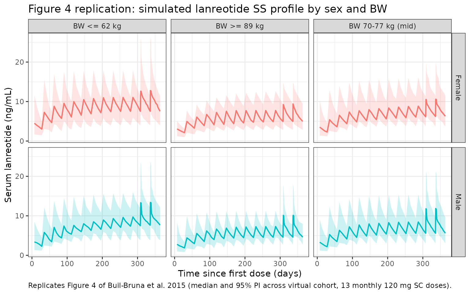
Inspect the parallel-absorption signature near each dose
The typical-value profile makes the parallel-absorption signature
visible: a small D0-bounded zero-order ledge in the first
~3 days after each dose riding on top of the slow first-order
rise/decay.
sim_typical |>
  filter(id %in% c(1L), time <= 84) |>   # first three doses for one subject
  ggplot(aes(x = time, y = Cc)) +
  geom_line(linewidth = 0.7) +
  geom_vline(xintercept = dose_times[1:3], linetype = "dashed", alpha = 0.4) +
  labs(
    x       = "Time since first dose (days)",
    y       = "Serum lanreotide (ng/mL)",
    title   = "Parallel first- and zero-order absorption signature (typical-value subject)",
    caption = "Dashed lines mark Q4W 120 mg SC doses. Zero-order phase ends at dose-time + D0 (= 2.96 days)."
  ) +
  theme_bw()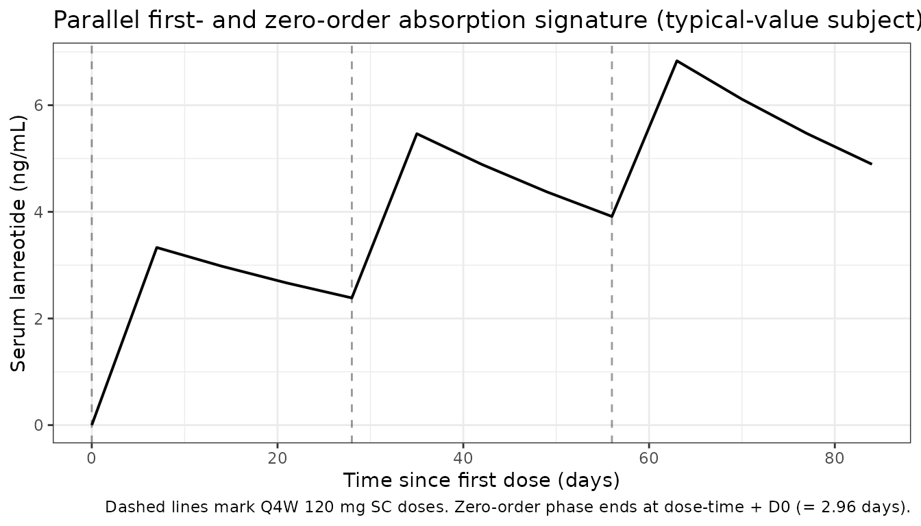
PKNCA validation
We compute steady-state pharmacokinetic descriptors (Cmin, Cmax, Cavg, AUCs) over the last dosing interval and compare against Buil-Bruna 2015 Table 3, which reports geometric mean and range for the same descriptors stratified by sex and body weight at the 120 mg dose level. The PKNCA formula groups by treatment to match the paper’s reporting units.
# Restrict NCA to the final SS interval [last_dose_t, end_time]
nca_conc <- sim |>
  filter(time >= last_dose_t, time <= end_time, !is.na(Cc), Cc > 0) |>
  select(id, time, Cc, sex_group, bw_group)

# One dose row per subject for the final dose
nca_dose <- dose_rows |>
  filter(time == last_dose_t) |>
  transmute(id, time, amt, sex_group, bw_group)
conc_obj <- PKNCAconc(nca_conc, Cc ~ time | sex_group + bw_group + id,
                      concu = "ng/mL", timeu = "day")
dose_obj <- PKNCAdose(nca_dose, amt ~ time | sex_group + bw_group + id,
                      doseu = "mg")

# AUC over [start_ss, start_ss + tau], plus Cmax, Tmax, Cmin, Cav
intervals <- data.frame(
  start    = last_dose_t,
  end      = end_time,
  cmax     = TRUE,
  tmax     = TRUE,
  cmin     = TRUE,
  auclast  = TRUE,
  cav      = TRUE
)

nca_data <- PKNCAdata(conc_obj, dose_obj, intervals = intervals)
nca_res  <- pk.nca(nca_data)
# Geometric-mean summary by overall, sex, and BW group, matching the
# stratifications in Buil-Bruna 2015 Table 3.
gmean <- function(x) exp(mean(log(x[is.finite(x) & x > 0])))

results_long <- as.data.frame(nca_res$result) |>
  filter(PPTESTCD %in% c("cmin", "cmax", "cav", "auclast")) |>
  inner_join(pop |> select(id, sex_group, bw_group),
             by = c("id", "sex_group", "bw_group"))

# Sex-only stratification
sex_tbl <- results_long |>
  group_by(sex_group, PPTESTCD) |>
  summarise(
    gmean = gmean(PPORRES),
    pmin  = min(PPORRES,    na.rm = TRUE),
    pmax  = max(PPORRES,    na.rm = TRUE),
    .groups = "drop"
  )

# BW-only stratification (Table 3 BW columns)
bw_tbl <- results_long |>
  group_by(bw_group, PPTESTCD) |>
  summarise(
    gmean = gmean(PPORRES),
    pmin  = min(PPORRES,    na.rm = TRUE),
    pmax  = max(PPORRES,    na.rm = TRUE),
    .groups = "drop"
  )

# Whole-population
whole_tbl <- results_long |>
  group_by(PPTESTCD) |>
  summarise(
    gmean = gmean(PPORRES),
    pmin  = min(PPORRES,    na.rm = TRUE),
    pmax  = max(PPORRES,    na.rm = TRUE),
    .groups = "drop"
  )

knitr::kable(whole_tbl, digits = 2, caption = "Simulated whole-population SS NCA (compare against Buil-Bruna 2015 Table 3 'Whole population').")| PPTESTCD | gmean | pmin | pmax |
|---|---|---|---|
| auclast | 220.42 | 53.77 | 457.06 |
| cav | 7.87 | 1.92 | 16.32 |
| cmax | 11.31 | 2.97 | 25.53 |
| cmin | 5.86 | 1.29 | 12.76 |
knitr::kable(sex_tbl, digits = 2, caption = "Simulated SS NCA by sex (compare against Table 3 'Males' / 'Females').")| sex_group | PPTESTCD | gmean | pmin | pmax |
|---|---|---|---|---|
| Female | auclast | 230.32 | 92.93 | 457.06 |
| Female | cav | 8.23 | 3.32 | 16.32 |
| Female | cmax | 10.98 | 3.64 | 25.53 |
| Female | cmin | 6.20 | 2.66 | 12.72 |
| Male | auclast | 212.43 | 53.77 | 451.63 |
| Male | cav | 7.59 | 1.92 | 16.13 |
| Male | cmax | 11.60 | 2.97 | 24.21 |
| Male | cmin | 5.59 | 1.29 | 12.76 |
knitr::kable(bw_tbl, digits = 2, caption = "Simulated SS NCA by BW band (compare against Table 3 BW columns).")| bw_group | PPTESTCD | gmean | pmin | pmax |
|---|---|---|---|---|
| BW 70-77 kg (mid) | auclast | 223.33 | 125.45 | 457.06 |
| BW 70-77 kg (mid) | cav | 7.98 | 4.48 | 16.32 |
| BW 70-77 kg (mid) | cmax | 11.58 | 5.49 | 25.53 |
| BW 70-77 kg (mid) | cmin | 5.84 | 1.29 | 12.76 |
| BW <= 62 kg | auclast | 268.40 | 142.84 | 428.01 |
| BW <= 62 kg | cav | 9.59 | 5.10 | 15.29 |
| BW <= 62 kg | cmax | 13.69 | 5.54 | 23.96 |
| BW <= 62 kg | cmin | 7.18 | 3.75 | 12.72 |
| BW >= 89 kg | auclast | 163.13 | 53.77 | 330.00 |
| BW >= 89 kg | cav | 5.83 | 1.92 | 11.79 |
| BW >= 89 kg | cmax | 8.14 | 2.97 | 18.00 |
| BW >= 89 kg | cmin | 4.57 | 1.66 | 8.17 |
Comparison against Buil-Bruna 2015 Table 3
Table 3 of the paper reports geometric mean (range) for Cmin, Cavg, Cmax (ng/mL), and AUCs (ug.day/L, numerically equal to ng.day/mL):
| Stratum | Cmin (ng/mL) | Cavg (ng/mL) | Cmax (ng/mL) | AUCs (ng.day/mL) |
|---|---|---|---|---|
| Whole population | 6.23 (0.3-14.7) | 8.35 (3.8-18.0) | 12.77 (4.2-63.8) | 231.5 (103.1-492.0) |
| Males | 5.5 (0.3-14.5) | 7.7 (4.5-17.9) | 13.7 (6-63.7) | 216 (124-490) |
| Females | 7 (2-14.7) | 9 (3.8-18) | 11.9 (4.2-40.2) | 247 (103-492) |
| BW <= 62 kg | 7.7 (2-14.7) | 10.3 (6.3-17.3) | 15.3 (7-63.7) | 285 (170-489) |
| BW 70-77 kg | 6.4 (3.5-12.4) | 8.3 (5.9-14.6) | 12.2 (6.8-31.8) | 228 (160-398) |
| BW >= 89 kg | 5.3 (2.8-14.5) | 6.8 (3.8-17.9) | 10.1 (4.2-23.6) | 188 (103-490) |
The simulated tables above should land in the same range. The direction of the body-weight effect (lower Cmax / Cavg / AUC for heavier patients) is mechanistic in the model (CL/F linear in WT) and must reproduce; sex differences are very small because the F1-on-sex effect is only 2.4% in absolute terms (Table 2 theta_SEX = -0.024 applied to the male indicator).
Assumptions and deviations
-
Absolute bioavailability F = 1 (structural anchor).
The paper declares F is not identifiable (Fig. 2 caption: “F absolute
bioavailability (not known and arbitrarily set to 1)”). All reported
parameters are therefore apparent (CL/F, Vd/F); the model faithfully
preserves this anchor by routing the F1 fraction into
depotand the F2 = 1 - F1 fraction intocentralso that F1 + F2 = -
F1 IPV close to its bound. Buil-Bruna 2015 Methods
state IPV was modeled exponentially. The reported IPV for F1 is 1.05% CV
(Table 2) applied to a typical value of 0.994 (females), which sits very
close to the structural upper bound F1 <= 1. Under exponential IIV a
meaningful fraction of simulated subjects can sample F1 > 1; in the
model the resulting F2 = 1 - F1 < 0 keeps mass balance intact (depot
delivers F1 * dose and
kzeroremoves the complementary excess from central over D0), but the F2 -> negative interpretation is non-physical. Stochastic simulations near this boundary are expected to be numerically robust because the magnitude of the out-of-bound excursion is tiny; users sensitive to the boundary should clip F1 to (0, 1] in the simulation post-processing. - Race / ethnicity not modeled. Buil-Bruna 2015 did not test RACE as a covariate because the cohort was predominantly White (Sect. 3.2). Fig. 5b confirmed retrospectively that observed Asian (n = 10) and Black/African American (n = 10) profiles fell within the population 90% PI. The virtual cohort here does not stratify by race.
- Sex split assumed 50/50. The paper does not tabulate sex proportions in the pooled population; per-study male/female counts are not given in the extractable Table 1 layout. The virtual cohort uses a 50/50 split for illustration.
- Body-weight distribution. Individual weights were not published. The virtual cohort draws WT from a log-normal with geometric mean 74 kg (the published median) and CV 22% (Buil-Bruna 2015 Table 1 pooled-CV row); the resulting BW band counts are not exactly the paper’s 20/50/80 percentile bins but cover the same range.
- Time-varying covariates not exercised. The paper applies the Wahlby et al. 2004 time-varying-covariate adjustment for BW changes during the study (Sect. 3.3.3); the virtual cohort holds WT constant at baseline. The reported impact of including time-varying BW was a -2LL reduction of 7.96 points with no change in IPV or other parameters, so the constant-WT approximation is a faithful simplification.
- NCA stratification approximates Table 3. The paper’s BW bands (<=62, 70-77, >=89 kg) correspond to the 20th, 50th, and 80th percentiles of the studied population (Methods Sect. 2.4.4). The virtual cohort uses the same numerical band edges; the resulting per-band sample sizes are determined by the log-normal sampling.