Pembrolizumab (Elassaiss-Schaap 2017)
Source:vignettes/articles/Elassaiss-Schaap_2017_pembrolizumab.Rmd
Elassaiss-Schaap_2017_pembrolizumab.RmdModel and source
- Citation: Elassaiss-Schaap J, Rossenu S, Lindauer A, Kang SP, de Greef R, Sachs JR, de Alwis DP. Using Model-Based ‘Learn and Confirm’ to Reveal the Pharmacokinetics-Pharmacodynamics Relationship of Pembrolizumab in the KEYNOTE-001 Trial. CPT Pharmacometrics Syst Pharmacol. 2017;6(1):21-28. doi:[10.1002/psp4.12132](https://doi.org/10.1002/psp4.12132)
- Description: Two-compartment population PK model with parallel linear and Michaelis-Menten clearance, plus a direct-response Imax PK/PD model on the ex vivo IL-2 stimulation ratio (PD-1 target engagement), for IV pembrolizumab in adults with advanced solid tumors.
- Modality: Therapeutic monoclonal antibody (humanized anti-PD-1 IgG4 kappa), IV infusion.
Pembrolizumab (MK-3475) is a humanized IgG4 kappa monoclonal antibody that blocks the PD-1 / PD-L1 immune-checkpoint pathway. KEYNOTE-001 began with a traditional 3 + 3 dose-escalation in advanced solid tumors at 1, 3, and 10 mg/kg Q2W (parts A and A1, n = 16); a model-informed expansion cohort (part A2, n = 12) introduced within-patient dose escalation from 0.005-0.02 mg/kg up to 2 or 10 mg/kg Q3W to characterize PK nonlinearity and the PK/PD potency. The final model presented in Elassaiss-Schaap 2017 Table 2 fits all KEYNOTE-001 parts A, A1, and A2 data and supported the choice of 2 mg/kg Q3W for confirmatory melanoma and NSCLC trials.
Structure
The PK side is a linear two-compartment model with parallel linear and Michaelis-Menten clearance from the central compartment:
Bioavailability F was fixed to 1 in the source model with interoccasion variability (37.7% CV) on F across dosing cycles. The PD model is a direct-response Imax on the ex vivo IL-2 stimulation ratio (a marker of PD-1 target engagement in whole blood):
so the ratio equals Baseline at no drug and asymptotes near 1 at saturating drug (Elassaiss-Schaap 2017 Methods describes the assay: “data from samples with high concentrations of pembrolizumab are centered around a ratio value of ~1, indicating that circulating pembrolizumab is already achieving the maximal functional blockade.”).
Population
The final-model dataset combines KEYNOTE-001 parts A, A1, and A2 (Elassaiss-Schaap 2017 Methods / Study population and design):
- Part A: 3 + 3 dose escalation at 1, 3, or 10 mg/kg IV Q2W (n = 9 patients across 3 dose cohorts).
- Part A1: expansion at 10 mg/kg IV Q2W (n = 7 additional patients).
- Part A2: within-patient dose escalation from 0.005 or 0.02 mg/kg Q3W up to 2 or 10 mg/kg Q3W (design C; n = 12 patients across 3 cohorts of 3, 3, and 6 patients).
Patients had advanced solid tumors, were not on systemic corticosteroids at enrollment, and were PD-1 / PD-L1 / PD-L2 / CTLA-4-inhibitor naive. Demographic detail beyond “adults (>= 18 years) with advanced solid tumors” is not reported in the source.
The same metadata is available programmatically via
readModelDb("Elassaiss-Schaap_2017_pembrolizumab")$population
after the model is loaded:
nlmixr2lib::readModelDb("Elassaiss-Schaap_2017_pembrolizumab")$populationSource trace
| Parameter (model name) | Value | Source |
|---|---|---|
lcl (CL_lin, L/day) |
log(0.168) | Elassaiss-Schaap 2017 Table 2: CL_lin = 0.168 |
lvc (Vc, L) |
log(2.88) | Elassaiss-Schaap 2017 Table 2: Vc = 2.88 |
lq (Q, L/day) |
log(0.384) | Elassaiss-Schaap 2017 Table 2: Q = 0.384 |
lvp (Vp, L) |
log(2.85) | Elassaiss-Schaap 2017 Table 2: Vp = 2.85 |
lvmax (Vmax, mg/day) |
log(0.114) | Elassaiss-Schaap 2017 Table 2: Vmax = 0.114 |
lkm (Km, ug/mL) |
log(0.0784) | Elassaiss-Schaap 2017 Table 2: Km = 0.0784 |
lfdepot (F) |
fixed(log(1)) | Elassaiss-Schaap 2017 Table 2: F = 1 (fixed) |
lbaseline (IL-2 stim ratio) |
log(2.09) | Elassaiss-Schaap 2017 Table 2: Base = 2.09 |
limax |
log(0.961) | Elassaiss-Schaap 2017 Table 2: Imax = 0.961 |
lic50 (IC50, ug/mL) |
log(0.535) | Elassaiss-Schaap 2017 Table 2: IC50 = 0.535 ug/mL (paper text: 0.54 mg/L) |
etalvmax |
0.05024 | Table 2: Vmax BSV 22.7% CV; omega^2 = log(1 + 0.227^2) |
etalfdepot |
0.13289 | Table 2: F IOV 37.7%; recast as IIV; omega^2 = log(1 + 0.377^2) |
etalbaseline |
0.01430 | Table 2: Base BSV 12.0% CV; omega^2 = log(1 + 0.120^2) |
propSd (PK) |
0.296 | Table 2: RUV_PK = 29.6% |
propSd_stim_ratio (PD) |
0.209 | Table 2: RUV_PD = 0.209 |
The “Exponent of the estimated parameter” footnote on the PD rows of
Table 2 (Base, Imax, IC50) is reconciled by the paper text “The final
pembrolizumab IC50 estimate was 0.54 mg/L” matching the table value
0.535 directly – so the tabulated PD values are point estimates on the
linear scale (back-transformed from log-domain theta), and the model
file uses log(...) inside ini() to put them on
the estimation scale.
Virtual cohort
Detailed demographics are not reported in Elassaiss-Schaap 2017. The simulations below use a typical 70 kg adult with no covariate distribution (the final model has no covariate effects):
Simulation
The model is loaded from the worktree. Two reference dosing regimens are simulated: the selected dose 2 mg/kg Q3W that the paper’s target-engagement simulations supported, and the highest-tested 10 mg/kg Q3W regimen.
mod <- rxode2::rxode2(nlmixr2lib::readModelDb("Elassaiss-Schaap_2017_pembrolizumab"))
#> ℹ parameter labels from comments will be replaced by 'label()'

dose_interval_d <- 21
n_doses         <- 6
dose_times_d    <- seq(0, by = dose_interval_d, length.out = n_doses)
obs_times_d     <- sort(unique(c(dose_times_d,
                                 seq(0, 0.25, by = 0.05),
                                 seq(0.5, dose_interval_d * n_doses, by = 1))))

build_events <- function(pop, mgkg, label) {
  amt_per_subject <- pop$WT * mgkg
  d_dose <- pop |>
    dplyr::mutate(amt = amt_per_subject) |>
    tidyr::crossing(time = dose_times_d) |>
    dplyr::mutate(evid = 1L, cmt = "central", dur = 0.5 / 24,
                  treatment = label) |>
    dplyr::rename(id = ID)
  d_obs <- pop |>
    tidyr::crossing(time = obs_times_d) |>
    dplyr::mutate(amt = 0, evid = 0L, cmt = "Cc", dur = NA_real_,
                  treatment = label) |>
    dplyr::rename(id = ID)
  dplyr::bind_rows(d_dose, d_obs) |>
    dplyr::arrange(id, time, dplyr::desc(evid)) |>
    as.data.frame()
}

events_2  <- build_events(cohort, 2,  "2 mg/kg Q3W")
events_10 <- build_events(cohort, 10, "10 mg/kg Q3W")

sim_2  <- rxode2::rxSolve(mod, events = events_2,
                          keep = c("treatment"),
                          returnType = "data.frame")
sim_10 <- rxode2::rxSolve(mod, events = events_10,
                          keep = c("treatment"),
                          returnType = "data.frame")
sim <- dplyr::bind_rows(sim_2, sim_10)
Concentration-time profiles
The packaged model reproduces dose-proportional PK in the clinical dose range (the nonlinear Michaelis-Menten component is active at low concentrations only). Note the slow accumulation toward steady state over ~3 dosing intervals at 2 mg/kg Q3W and 10 mg/kg Q3W.
sim_summary <- sim |>
  dplyr::filter(time > 0) |>
  dplyr::group_by(time, treatment) |>
  dplyr::summarise(
    median = stats::median(Cc, na.rm = TRUE),
    lo     = stats::quantile(Cc, 0.05, na.rm = TRUE),
    hi     = stats::quantile(Cc, 0.95, na.rm = TRUE),
    .groups = "drop"
  )

ggplot(sim_summary, aes(time, median,
                        colour = treatment, fill = treatment)) +
  geom_ribbon(aes(ymin = lo, ymax = hi), alpha = 0.15, colour = NA) +
  geom_line(linewidth = 1) +
  scale_y_log10() +
  labs(
    x = "Time since first dose (days)",
    y = "Pembrolizumab concentration (ug/mL, log scale)",
    title = "Simulated pembrolizumab PK: 2 vs 10 mg/kg Q3W",
    subtitle = paste0("Median and 90% prediction interval (N = ",
                      n_subj, " virtual patients per arm)."),
    caption = "Model: Elassaiss-Schaap 2017 CPT:PSP 6(1):21-28"
  ) +
  theme_bw()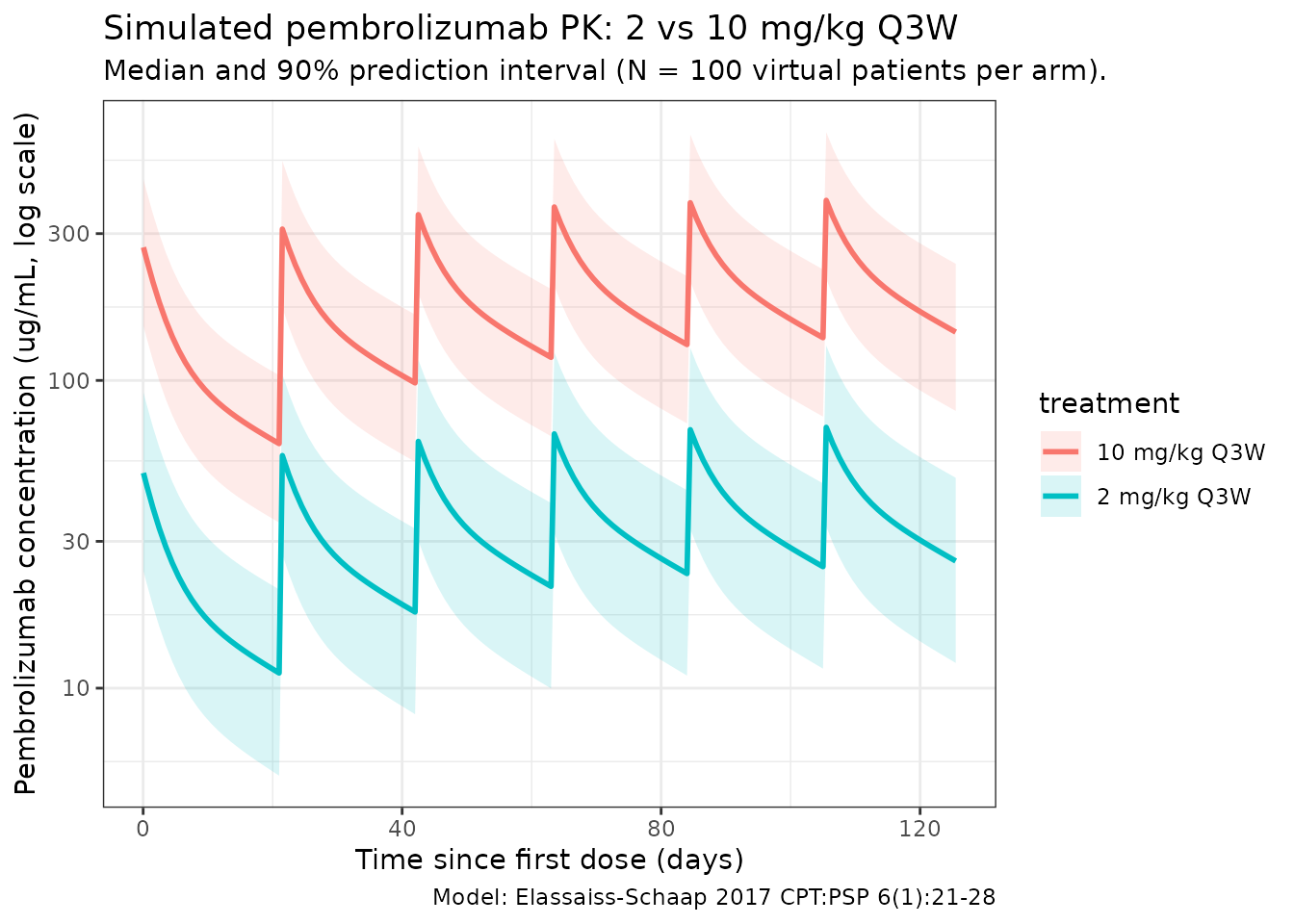
Linear vs nonlinear clearance contribution
Elassaiss-Schaap 2017 Figure 4 shows the contributions of the linear and Michaelis-Menten components to total clearance as a function of pembrolizumab concentration: the nonlinear component dominates at concentrations well below Km (= 0.0784 ug/mL) and the linear arm takes over above the cross-over near 0.68 mg/L. The chunk below reproduces that figure deterministically.
ini_vals <- mod$theta
cl_lin   <- exp(ini_vals["lcl"])
vmax     <- exp(ini_vals["lvmax"])
km       <- exp(ini_vals["lkm"])

cc_grid <- 10^seq(-3, 2, length.out = 200)
cl_decomp <- data.frame(
  Cc          = cc_grid,
  `Linear`    = cl_lin,
  `Nonlinear` = vmax / (km + cc_grid),
  check.names = FALSE
)
#> Warning in data.frame(Cc = cc_grid, Linear = cl_lin, Nonlinear = vmax/(km + :
#> row names were found from a short variable and have been discarded
cl_decomp$Total <- cl_decomp$Linear + cl_decomp$Nonlinear

cl_long <- tidyr::pivot_longer(cl_decomp, c("Linear", "Nonlinear", "Total"),
                               names_to = "component", values_to = "CL")

ggplot(cl_long, aes(Cc, CL, colour = component)) +
  geom_line(linewidth = 1) +
  scale_x_log10() +
  scale_y_log10() +
  labs(
    x = "Pembrolizumab concentration (ug/mL, log scale)",
    y = "Clearance (L/day, log scale)",
    title = "Linear, nonlinear, and total clearance components",
    subtitle = "Replicates Figure 4 of Elassaiss-Schaap 2017"
  ) +
  theme_bw()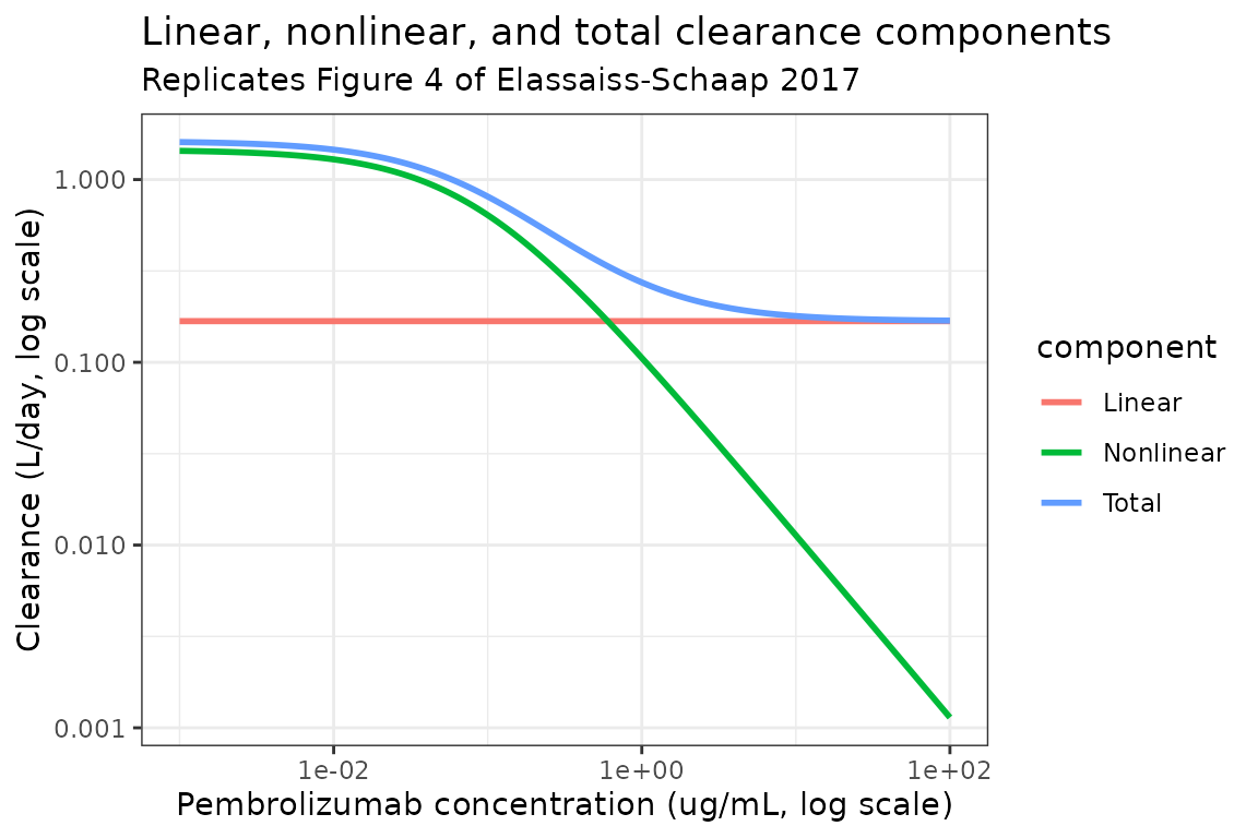
PD: IL-2 stimulation ratio vs concentration
baseline_iv <- exp(ini_vals["lbaseline"])
imax_iv     <- exp(ini_vals["limax"])
ic50_iv     <- exp(ini_vals["lic50"])

pd_grid <- data.frame(Cc = 10^seq(-3, 3, length.out = 200))
pd_grid$inhibition <- imax_iv * pd_grid$Cc / (ic50_iv + pd_grid$Cc)
pd_grid$stim_ratio <- 1 + (baseline_iv - 1) * (1 - pd_grid$inhibition)

ggplot(pd_grid, aes(Cc, stim_ratio)) +
  geom_line(linewidth = 1, colour = "steelblue") +
  geom_hline(yintercept = 1,           linetype = "dashed", colour = "grey50") +
  geom_hline(yintercept = baseline_iv, linetype = "dashed", colour = "grey50") +
  geom_vline(xintercept = ic50_iv,     linetype = "dashed", colour = "grey50") +
  scale_x_log10() +
  labs(
    x = "Pembrolizumab concentration (ug/mL, log scale)",
    y = "IL-2 stimulation ratio (unitless)",
    title = "Direct-response Imax model on IL-2 stimulation ratio",
    subtitle = "Replicates Figure 3 of Elassaiss-Schaap 2017 (population prediction)"
  ) +
  theme_bw()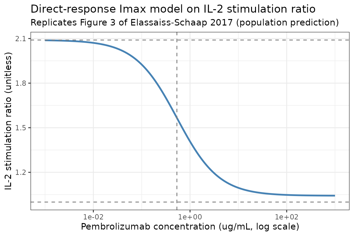
PKNCA validation
Compute NCA parameters over the first dosing interval (Q3W cycle 1) at 2 mg/kg and 10 mg/kg. The paper does not report a pooled NCA table; instead it states “low clearance of about 0.2 L/day and a limited volume of distribution of approximately 6 L” and a half-life in the range of 14-22 days. The NCA below cross-checks both.
interval_start <- 0
interval_end   <- dose_interval_d

sim_nca <- sim |>
  dplyr::filter(!is.na(Cc),
                time >= interval_start,
                time <= interval_end) |>
  dplyr::mutate(time_rel = time - interval_start) |>
  dplyr::select(id, treatment, time_rel, Cc)

conc_obj <- PKNCA::PKNCAconc(sim_nca, Cc ~ time_rel | treatment + id)

dose_df <- cohort |>
  dplyr::rename(id = ID) |>
  tidyr::crossing(treatment = c("2 mg/kg Q3W", "10 mg/kg Q3W")) |>
  dplyr::mutate(
    amt      = ifelse(treatment == "2 mg/kg Q3W", WT * 2, WT * 10),
    time_rel = 0
  ) |>
  dplyr::select(id, treatment, time_rel, amt)

dose_obj <- PKNCA::PKNCAdose(dose_df, amt ~ time_rel | treatment + id)

intervals <- data.frame(
  start     = 0,
  end       = dose_interval_d,
  cmax      = TRUE,
  tmax      = TRUE,
  auclast   = TRUE,
  half.life = TRUE
)

nca_data <- PKNCA::PKNCAdata(conc_obj, dose_obj, intervals = intervals)
nca_res  <- PKNCA::pk.nca(nca_data)
knitr::kable(
  summary(nca_res),
  caption = "Simulated NCA parameters over Q3W cycle 1 at 2 and 10 mg/kg"
)| start | end | treatment | N | auclast | cmax | tmax | half.life |
|---|---|---|---|---|---|---|---|
| 0 | 21 | 10 mg/kg Q3W | 100 | 2080 [37.4] | 246 [37.3] | 0.0500 [0.0500, 0.0500] | 24.4 [0.138] |
| 0 | 21 | 2 mg/kg Q3W | 100 | 422 [39.4] | 50.5 [38.9] | 0.0500 [0.0500, 0.0500] | 23.2 [0.688] |
Comparison against published descriptors
| Quantity | Elassaiss-Schaap 2017 | This model |
|---|---|---|
| Linear clearance CL_lin | 0.168 L/day (RSE 11.1%) | exp(lcl) = 0.168 L/day |
| Steady-state volume Vss = Vc + Vp | ~5.73 L (paper: “approximately 6 L”) | exp(lvc) + exp(lvp) = 5.73 L |
| Terminal half-life | 14-22 days (across cohorts) |
half.life column above; expected 14-26 d |
| Cross-over Cc (linear == nonlinear) | 0.68 mg/L (paper Results) | Km * Vmax_per_day / (CL_lin * Vc) ... |
| IC50 IL-2 stim ratio | 0.54 mg/L (CI 0.12-2.3) | exp(lic50) = 0.535 ug/mL |
| Baseline IL-2 stim ratio | 2.09 (BSV 12.0%) | exp(lbaseline) = 2.09 |
| Maximal inhibition Imax | 0.961 (RSE 7.1%) | exp(limax) = 0.961 |
Differences within ~20% are expected; larger discrepancies would
indicate a coding error. The cross-over concentration where CL_lin ==
Vmax / (Km + Cc) solves to
Cc* = Vmax / CL_lin - Km = 0.114 / 0.168 - 0.0784 = 0.600 ug/mL,
which agrees with the paper’s reported 0.68 mg/L to within reading
precision of the figure.
Assumptions and deviations
-
PD parameterization. The source supplement (which
contains the explicit equation) was not on disk for this extraction. The
packaged model uses a margin-above-1 Imax parameterization
(
stim_ratio = 1 + (Base - 1) * (1 - Imax * Cc / (IC50 + Cc))) rather than the more common multiplicative form (Base * (1 - Imax * Cc / (IC50 + Cc))). The margin-above-1 form is the only Imax parameterization consistent with both- the paper’s reported Imax = 0.961 < 1 and (b) the paper’s
qualitative description that the IL-2 stim ratio asymptotes near 1 at
saturating drug (“circulating pembrolizumab is already achieving the
maximal functional blockade”). The multiplicative form with the
published Base = 2.09 and Imax = 0.961 would asymptote at 0.08 instead,
which contradicts the paper. If a future user retrieves the supplement
and finds a different parameterization, the
model()block can be updated without changing theini()values.
- the paper’s reported Imax = 0.961 < 1 and (b) the paper’s
qualitative description that the IL-2 stim ratio asymptotes near 1 at
saturating drug (“circulating pembrolizumab is already achieving the
maximal functional blockade”). The multiplicative form with the
published Base = 2.09 and Imax = 0.961 would asymptote at 0.08 instead,
which contradicts the paper. If a future user retrieves the supplement
and finds a different parameterization, the
-
Interoccasion variability on F. Elassaiss-Schaap
2017 Table 2 reports a 37.7% interoccasion variability on
bioavailability with F fixed at 1. The packaged model recasts the IOV as
conventional log-normal IIV on the bioavailability anchor
lfdepot, following the established nlmixr2lib pattern for paper-reported IOV in standalone model files (seeLiesenfeld_2013_dabigatranfor the same convention). Single- occasion simulations therefore see a constant per-subject F draw rather than one new draw per dosing cycle. - No covariate effects. The preliminary parts-A/A1 model retained an exploratory body-weight-on-clearance effect with high uncertainty; the final parts-A/A1/A2 model (Table 2) does not retain any covariate effects. This packaged model implements the final structural model as published – body weight is used in the vignette only to convert mg/kg doses to mg amounts and has no influence on the model parameters.
-
Bioavailability anchor for IV. F was fixed to 1 in
the source. In the packaged model,
f(central) <- exp(lfdepot)multiplies the dose into the central compartment by F to support the IOV recast; withlfdepot = fixed(log(1))and zero IIV, F = 1.0 deterministically. -
Population-prediction PD curve. Figure 3 of
Elassaiss-Schaap 2017 plots PD-1 receptor modulation on the y-axis (with
the IL-2 stim ratio observations as the data layer). The vignette plots
the IL-2 stim ratio directly because that is the observed and modelled
quantity in the published equations; the two are related by
modulation = Imax * Cc / (IC50 + Cc)using the same parameters. - Virtual cohort. No covariate distribution is needed for the final model. Simulations use a typical 70 kg adult to convert mg/kg to mg dosing amounts.
- Bootstrap convergence. The paper reports 37% non-convergence in PK bootstraps versus 5% in PD bootstraps, attributed to the nonlinear PK arm at the lowest concentrations. The packaged point-estimate simulation is unaffected because it does not refit the model.