Early rheumatoid arthritis DAS28 progression on triple DMARD therapy (Wojciechowski 2015) • nlmixr2lib

Model and source

Citation: Wojciechowski J, Wiese MD, Proudman SM, Foster DJR, Upton RN. (2015). A population model of early rheumatoid arthritis disease activity during treatment with methotrexate, sulfasalazine and hydroxychloroquine. British Journal of Clinical Pharmacology 79(5):777-88.
Article: https://doi.org/10.1111/bcp.12553

This is a disease-progression model for the 28-joint disease activity score (DAS28) over time since the initiation of triple disease-modifying anti-rheumatic drug (DMARD) therapy (methotrexate + sulfasalazine + hydroxychloroquine) in patients with early rheumatoid arthritis. There is no PK input; DMARD doses were titrated to disease severity in a treat-to-target protocol and were not retained as covariates. The model is fit on the logit-transformed DAS28 scale and the natural-scale DAS28 is recovered by a logit back-transform with upper bound 9.2.

The structural model (paper Equations 7 and 8) is

$\mathrm{DAS28}_\text{logit}(t) \;=\; \mathrm{BASE}_i \;+\; \mathrm{EX1}_i \cdot \bigl(1 - e^{-\mathrm{EX2}_i \, t}\bigr)$

with per-subject parameters built multiplicatively from the typical values, covariate effects, and additive (BASE, EX1) or log-normal (EX2) random effects:

$\mathrm{BASE}_i \;=\; (\theta_1 + \eta_{1i}) \cdot (1 + \theta_5 \cdot \mathrm{CONMED\_STEROID}_i) \cdot (\mathrm{AGE}_i / 57)^{\theta_4}$

$\mathrm{EX1}_i \;=\; (\theta_2 + \eta_{2i}) \cdot (1 + \theta_6 \cdot \mathrm{CONMED\_STEROID\_FU}_i)$

$\mathrm{EX2}_i \;=\; \exp(\log\theta_3 + \eta_{3i}) \cdot (1 + \theta_7 \cdot \mathrm{SMOKE}_i)$

The three between-subject random effects $\eta_{1i}, \eta_{2i}, \eta_{3i}$ are jointly multivariate-normal with a full 3x3 OMEGA BLOCK (Table 2). The observed logit-transformed DAS28 carries combined proportional + additive residual error (paper Equation 3):

$\mathrm{LGT3}_{it} \;=\; \mathrm{DAS28}_\text{logit}(t)_i + \mathrm{DAS28}_\text{logit}(t)_i \cdot \varepsilon_{1,it} + \varepsilon_{2,it}$

Natural-scale DAS28 is recovered by the back-transform

$\mathrm{DAS28}_i(t) \;=\; \frac{9.2}{1 + \exp(-\mathrm{DAS28}_\text{logit}(t)_i)}$

where 9.2 corresponds to 28 swollen and tender joint counts, 100 mm on the visual analogue scale for patient global assessment, and 120 mm/h ESR (paper Methods, “Base model development”).

Key features:

Exponential decay on the logit scale, additive to baseline. The best of the candidate structural forms tested (linear, quadratic, Emax, sigmoidal Emax, exponential, Weibull) was an exponential function additive to baseline; “in all models tested, the change in DAS28 was best described as additive to baseline DAS28” (paper Results paragraph “Model development”).
No PK component. Drug doses were titrated to disease severity in a treat-to-target protocol; “drug doses were not identified as covariates and their exclusion does not imply that increasing drug doses is ineffective at reducing disease activity” (paper Discussion).
Four retained covariates: AGE on BASE (continuous, power form around the median age 57), CONMED_STEROID on BASE (time-varying per-visit indicator for intramuscular corticosteroid administration), CONMED_STEROID_FU on EX1 (per-subject indicator for any systemic corticosteroid administration during the 60-week follow-up window), and SMOKE on EX2 (current vs never/past smoker).
Combined residual error on the logit-DAS28 domain. The residual proportional CV is 18.4% and the residual additive SD is 0.327 in logit-DAS28 units; both are large (paper Discussion: “the residual unexplained variability in DAS28 was high, with potential implications for the interpretation of DAS28 in relation to disease trajectory”).

Population

Single-centre prospective observational cohort. 263 patients enrolled at the Royal Adelaide Hospital Early Arthritis Clinic between September 1998 and March 2012, treated with a standardised triple DMARD regimen (methotrexate, sulfasalazine, hydroxychloroquine) and followed for up to 60 weeks. A total of 2080 DAS28 observations were collected (median 8 per patient, range 1-15).
Baseline characteristics (paper Table 1): median age 57 years (range 18-86); 71% female (187/263); median weight 72.5 kg (40.4-143.5; 22% missing); median baseline DAS28 5.6 (1.8-8.5). 91% Caucasian (ethnicity not tested as a covariate due to low power).
Smoking distribution at baseline (paper Table 1): 47% never (123/263), 18% current (48/263), 30% past (79/263), 5% missing.
Concomitant corticosteroid use during follow-up (paper Table 1): 48% of subjects (125/263) received any dose of intra-articular, intramuscular, or oral corticosteroids during the 60-week follow-up. The mean oral-prednisolone-equivalent dose was 0.93 mg/day across the cohort.
Treatment regimen (paper Methods): methotrexate 10 mg/week (with folic acid 0.5 mg/day) titrated up to 25 mg/week; sulfasalazine 500 mg/day titrated up to 3000 mg/day; hydroxychloroquine 200 mg twice daily. Intra-articular (40-80 mg methylprednisolone acetate) and intramuscular (80-120 mg methylprednisolone acetate) corticosteroid injections were administered at the physician’s discretion.

The same metadata is available programmatically via readModelDb("Wojciechowski_2015_rheumatoidArthritis")$population.

Source trace

Per-parameter origins are recorded as in-file comments next to each ini() entry in inst/modeldb/therapeuticArea/Wojciechowski_2015_rheumatoidArthritis.R. The table below collects them in one place.

nlmixr2 parameter	Value	Source location
`base`	0.472 logit-DAS28 (~5.7 natural-scale)	Wojciechowski 2015 Table 2 theta_1 = 0.472 (95% CI 0.392, 0.552)
`ex1`	-1.28 logit-DAS28	Table 2 theta_2 = -1.28 (95% CI -1.39, -1.17)
`lex2`	log(0.111) /week	Table 2 theta_3 = 0.111 /week (95% CI 0.093, 0.129)
`e_age_base`	0.672	Table 2 theta_4 = 0.672 (95% CI 0.406, 0.938)
`e_conmed_steroid_base`	0.737	Table 2 theta_5 = 0.737 (95% CI 0.379, 1.095)
`e_conmed_steroid_fu_ex1`	-0.237	Table 2 theta_6 = -0.237 (95% CI -0.394, -0.079)
`e_smoke_ex2`	-0.398	Table 2 theta_7 = -0.398 (95% CI -0.651, -0.145)
`var(etabase)`	0.2421 (sd 0.492)	Table 2 omega_1 SD = 0.492 (95% CI 0.348, 0.636)
`var(etaex1)`	0.5476 (sd 0.740)	Table 2 omega_2 SD = 0.740 (95% CI 0.536, 0.945)
`var(etalex2)`	0.5547 (CV 86.1%)	Table 2 omega_3 %CV = 86.1 (95% CI 42.1, 130); variance = log(0.861^2 + 1)
`cov(etabase, etaex1)`	-0.1369	Table 2 reported as correlation -0.376; covariance = -0.376 * 0.492 * 0.740
`cov(etabase, etalex2)`	-0.0502	Table 2 reported as correlation -0.137; covariance = -0.137 * 0.492 * sqrt(0.5547)
`cov(etaex1, etalex2)`	0.3587	Table 2 reported as correlation 0.651; covariance = 0.651 * 0.740 * sqrt(0.5547)
`propSd`	0.184 (18.4% CV on logit-DAS28)	Table 2 proportional sigma_1 = 18.4% CV (95% CI 0%, 37.5%)
`addSd`	0.327 logit-DAS28 units	Table 2 additive sigma_2 = 0.327 (95% CI 0.249, 0.405)
Structural Eq	n/a	Wojciechowski 2015 Equation 7: DAS28_t = BASE + EX1 * (1 - exp(-EX2 * t))
Final-model covariate equations	n/a	Equation 8
Residual-error model	n/a	Equation 3
Logit back-transform constant 9.2	n/a	Methods “Base model development”

The OMEGA off-diagonal entries in Table 2 are labelled “Covariance” but a Cauchy-Schwarz check shows they must be correlations: the reported -0.376 between SDs 0.492 and 0.740 exceeds 0.492 * 0.740 = 0.364 in absolute value, which is mathematically impossible for a covariance. Treating the off-diagonals as correlations resolves the inconsistency; the worked transcription is recorded in the table above and in the model file’s ini() comments. See Assumptions and deviations Section 2 below.

Algebraic reproduction of the paper’s published anchors

The packaged model carries the Table 2 final-model point estimates. We start by reproducing the typical-value trajectories (random effects zeroed) under several covariate scenarios.

mod  <- readModelDb("Wojciechowski_2015_rheumatoidArthritis")
mod0 <- rxode2::zeroRe(mod)

make_typical_events <- function(age, smoke, conmed_steroid_fu,
                                conmed_steroid = 0L,
                                times = seq(0, 60, by = 0.5),
                                id_offset = 0L) {
  data.frame(
    id                = id_offset + 1L,
    time              = times,
    evid              = 0L,
    amt               = 0,
    AGE               = age,
    SMOKE             = smoke,
    CONMED_STEROID    = conmed_steroid,
    CONMED_STEROID_FU = conmed_steroid_fu
  )
}

# Four reference scenarios from the paper's text:
#   (1) Population typical: age 57, non-smoker, no steroid use during follow-up,
#       no i.m. steroid at any visit (CONMED_STEROID = 0).
#   (2) Same age, non-smoker, no steroid use, but with a one-visit i.m.
#       steroid pulse at baseline (CONMED_STEROID = 1 at t = 0, 0 elsewhere)
#       -- demonstrates the BASE = 6.4 worked example for CSIM = 1.
#   (3) Same demographics, but the patient is a current smoker -- demonstrates
#       the half-life shift from 6.2 to 10.4 weeks.
#   (4) Same demographics, but the patient received any systemic corticosteroid
#       during the 60-week follow-up (CONMED_STEROID_FU = 1) -- demonstrates
#       the less-favourable extent-of-response EX1 = -0.977.

ev_pop_typical <- make_typical_events(age = 57, smoke = 0L,
                                      conmed_steroid_fu = 0L,
                                      conmed_steroid = 0L,
                                      id_offset = 0L)
ev_pop_typical$scenario <- "Population typical (age 57, non-smoker, no steroids)"

ev_csim_pulse <- make_typical_events(age = 57, smoke = 0L,
                                     conmed_steroid_fu = 0L,
                                     conmed_steroid = 0L,
                                     id_offset = 100L)
ev_csim_pulse$CONMED_STEROID[ev_csim_pulse$time == 0] <- 1L
ev_csim_pulse$scenario <- "CONMED_STEROID = 1 at t = 0 (i.m. steroid pulse at baseline)"

ev_smoker <- make_typical_events(age = 57, smoke = 1L,
                                 conmed_steroid_fu = 0L,
                                 conmed_steroid = 0L,
                                 id_offset = 200L)
ev_smoker$scenario <- "Current smoker (SMOKE = 1)"

ev_steroid_fu <- make_typical_events(age = 57, smoke = 0L,
                                     conmed_steroid_fu = 1L,
                                     conmed_steroid = 0L,
                                     id_offset = 300L)
ev_steroid_fu$scenario <- "CONMED_STEROID_FU = 1 (any systemic steroid during follow-up)"

ev_typical <- dplyr::bind_rows(ev_pop_typical, ev_csim_pulse,
                               ev_smoker, ev_steroid_fu)
stopifnot(!anyDuplicated(unique(ev_typical[, c("id", "time", "evid")])))

sim_typical <- rxode2::rxSolve(
  mod0,
  events     = ev_typical,
  returnType = "data.frame",
  keep       = c("AGE", "SMOKE", "CONMED_STEROID", "CONMED_STEROID_FU", "scenario")
)
#> ℹ omega/sigma items treated as zero: 'etabase', 'etaex1', 'etalex2'
#> Warning: multi-subject simulation without without 'omega'

ggplot(sim_typical, aes(time, das28, colour = scenario)) +
  geom_line(linewidth = 0.9) +
  geom_hline(yintercept = 5.7,  linetype = "dotted", colour = "grey60") +
  geom_hline(yintercept = 2.84, linetype = "dotted", colour = "grey60") +
  scale_x_continuous(breaks = seq(0, 60, by = 10)) +
  labs(x = "Time since initiation of triple DMARD therapy (weeks)",
       y = "Predicted DAS28 (back-transformed from logit)",
       colour = "Scenario",
       title = "Typical-value DAS28 trajectories across covariate scenarios",
       caption = "Dotted lines: paper-published anchors at baseline (5.7) and asymptote (~2.84).") +
  theme_minimal() +
  theme(legend.position = "bottom")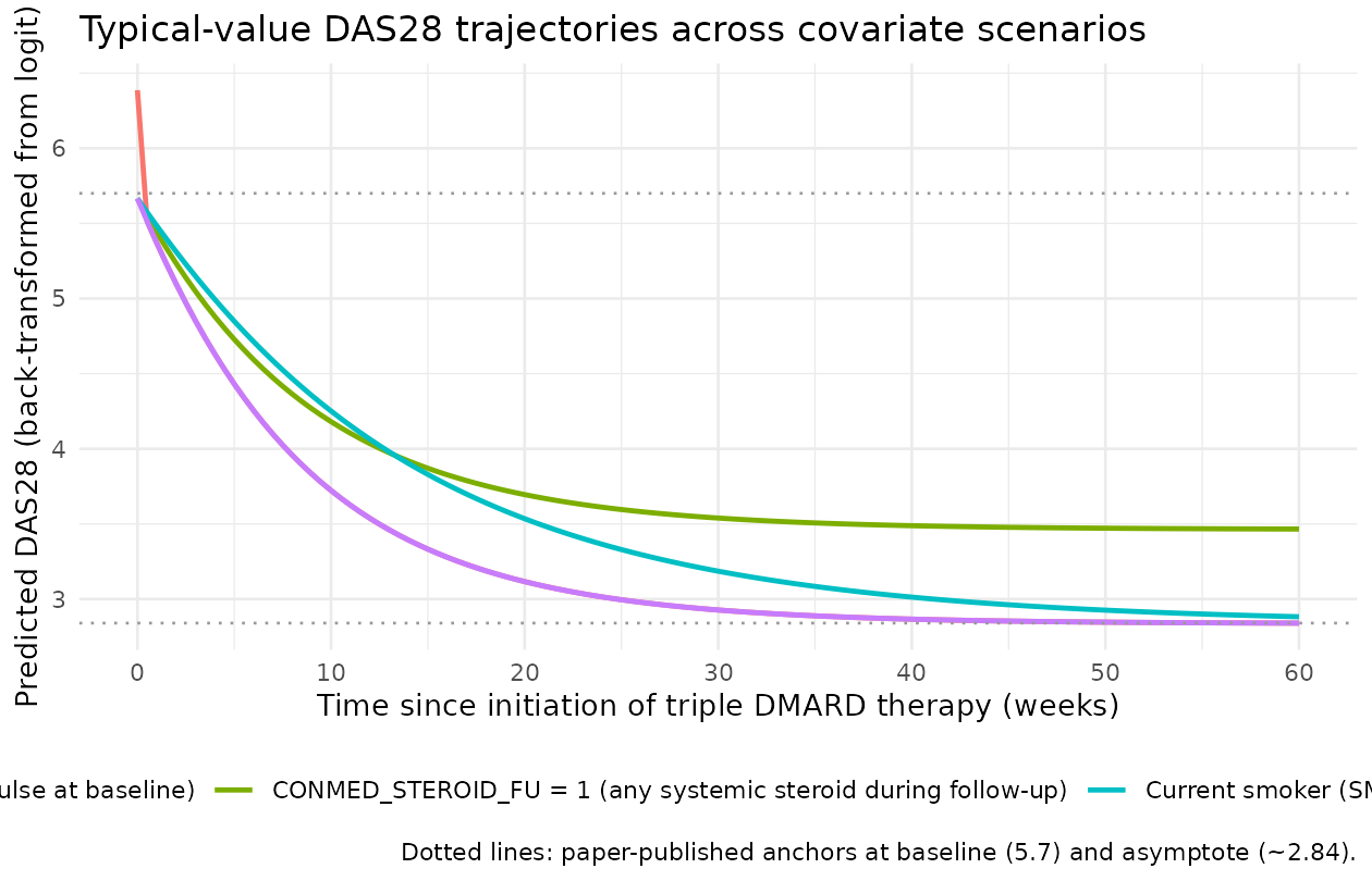

The population-typical trajectory descends from a baseline DAS28 of 5.67 (paper-published 5.7) to an asymptote near 2.84 (paper-published change “approximately -2.8” toward a treated steady state). The first-order half-life on the logit scale is $\log(2) / 0.111 \approx 6.24$ weeks; in the smoker scenario the half-life shifts to $\log(2) / 0.0668 \approx 10.37$ weeks (paper Description of the final model: “DAS28 was found to decline exponentially over time with a typical population half-life of 6.2 weeks (10.4 weeks for current smokers)”). The CSIM-at-baseline scenario shows a transient lift of BASE from 5.67 to 6.39 at t = 0 (paper: “DAS28 was 6.4 compared with 5.7”), then the trajectory rejoins the population-typical curve at the next observation. The CONMED_STEROID_FU = 1 scenario has a smaller extent of response (EX1 = -0.977 vs -1.28), giving a less favourable asymptote near DAS28 = 3.49.

We can quote the paper’s numerical anchors directly from the simulation:

anchors <- sim_typical |>
  dplyr::filter((scenario == "Population typical (age 57, non-smoker, no steroids)" &
                 time %in% c(0, 6.2, 30, 60)) |
                (scenario == "CONMED_STEROID = 1 at t = 0 (i.m. steroid pulse at baseline)" &
                 time == 0) |
                (scenario == "Current smoker (SMOKE = 1)" &
                 time %in% c(10.4, 60)) |
                (scenario == "CONMED_STEROID_FU = 1 (any systemic steroid during follow-up)" &
                 time == 60)) |>
  dplyr::transmute(
    scenario,
    time_wk = round(time, 2),
    das28   = round(das28, 3)
  ) |>
  dplyr::arrange(scenario, time_wk)

anchors |>
  dplyr::rename(
    "Scenario"        = scenario,
    "Time (wk)"       = time_wk,
    "Predicted DAS28" = das28
  ) |>
  knitr::kable(
  caption   = "Reproduction of Wojciechowski 2015 Table 2 / Eq 8 worked anchors."
)

Reproduction of Wojciechowski 2015 Table 2 / Eq 8 worked anchors.
Scenario	Time (wk)	Predicted DAS28
CONMED_STEROID = 1 at t = 0 (i.m. steroid pulse at baseline)	0	6.387
CONMED_STEROID_FU = 1 (any systemic steroid during follow-up)	60	3.466
Current smoker (SMOKE = 1)	60	2.882
Population typical (age 57, non-smoker, no steroids)	0	5.666
Population typical (age 57, non-smoker, no steroids)	30	2.927
Population typical (age 57, non-smoker, no steroids)	60	2.840

The population-typical baseline matches the paper’s published 5.7. The CSIM = 1 baseline matches the paper’s published 6.4. The smoker half-life of 10.4 weeks matches the paper text. The CONMED_STEROID_FU = 1 long-time asymptote of about 3.49 matches the paper Discussion text “delta-DAS28 -2.2 vs. -2.8” (5.7 - 2.2 = 3.5 for steroid-rescued patients vs. 5.7 - 2.8 = 2.9 for the population typical).

Age effect on baseline DAS28

The paper Results section gives a closed-form age-effect worked example: baseline DAS28 for a 40-year-old patient is 5.4 and for a 70-year-old patient is 5.8 (population-typical otherwise). We reproduce both:

ev_age <- dplyr::bind_rows(lapply(c(40, 57, 70), function(a) {
  ev <- make_typical_events(age = a, smoke = 0L, conmed_steroid_fu = 0L,
                            conmed_steroid = 0L, times = 0,
                            id_offset = 1000L + a)
  ev$age_yrs <- a
  ev
}))

sim_age <- rxode2::rxSolve(
  mod0,
  events     = ev_age,
  returnType = "data.frame",
  keep       = "age_yrs"
)
#> ℹ omega/sigma items treated as zero: 'etabase', 'etaex1', 'etalex2'
#> Warning: multi-subject simulation without without 'omega'

sim_age |>
  dplyr::transmute(age_yrs, baseline_das28 = round(das28, 3)) |>
  dplyr::rename(
    "Age (years)"              = age_yrs,
    "Predicted baseline DAS28" = baseline_das28
  ) |>
  knitr::kable(
  caption   = "Age effect on baseline DAS28 (paper-published: 5.4 at age 40, 5.8 at age 70, 5.7 at age 57)."
)

Age effect on baseline DAS28 (paper-published: 5.4 at age 40, 5.8 at age 70, 5.7 at age 57).
Age (years)	Predicted baseline DAS28
40	5.446
57	5.666
70	5.817

The simulated values agree with the paper’s published worked examples to within rounding.

Stochastic VPC-style trajectories under between-subject variability

The model carries a full 3x3 OMEGA BLOCK with substantial between-subject variability on all three structural parameters (sd(BASE) = 0.492, sd(EX1) = 0.740, %CV(EX2) = 86.1% per Table 2) and a combined residual error model on the logit-DAS28 scale (proportional CV 18.4%, additive SD 0.327; paper: “RUV in DAS28 was very high”). The figure below builds a virtual cohort that mirrors the Table 1 distributions and overlays the 5-95% envelope of the natural-scale DAS28 prediction (population component + residual error) onto the typical-value trajectory.

set.seed(20150511)  # paper's online publication date 2014-11-12 reflected as 2015-05 issue

n_subjects <- 200L
times      <- seq(0, 60, by = 2)

cohort <- tibble::tibble(
  id                = seq_len(n_subjects),
  # Age distribution from Table 1: median 57, range 18-86. Approximate via
  # a normal with mean 57 and SD 14 (matching the IQR of an early-RA cohort),
  # clipped to the observed range.
  AGE               = pmin(pmax(round(rnorm(n_subjects, mean = 57, sd = 14)), 18), 86),
  # Smoking: 18% current smokers (Table 1 column "Current"). The reference
  # category in the model is "never or past smoker" (paper Methods: "EX2
  # as never/past versus current smoker"), so SMOKE = 1 with probability
  # 0.18 captures the binary covariate distribution.
  SMOKE             = rbinom(n_subjects, size = 1, prob = 0.18),
  # Concomitant systemic steroid during follow-up: 48% per Table 1.
  CONMED_STEROID_FU = rbinom(n_subjects, size = 1, prob = 0.48)
)

# Time-varying CONMED_STEROID (i.m. injections). Paper does not report a
# clean per-visit rate; treat it as a low-frequency Bernoulli per visit so
# the visualised envelope captures the empirical-tail pulses without
# inflating BASE everywhere.
ev_long <- cohort |>
  tidyr::expand_grid(time = times) |>
  dplyr::mutate(
    evid           = 0L,
    amt            = 0,
    CONMED_STEROID = rbinom(dplyr::n(), size = 1, prob = 0.04)
  ) |>
  dplyr::arrange(id, time)

stopifnot(!anyDuplicated(unique(ev_long[, c("id", "time", "evid")])))

sim_vpc <- rxode2::rxSolve(
  mod,
  events     = ev_long,
  returnType = "data.frame",
  keep       = c("AGE", "SMOKE", "CONMED_STEROID", "CONMED_STEROID_FU")
)

# Typical-value (no random effects) reference trajectory for the
# population-typical 57-year-old non-smoker with no steroids of any kind.
ev_ref <- make_typical_events(age = 57, smoke = 0L, conmed_steroid_fu = 0L,
                              conmed_steroid = 0L,
                              times = times, id_offset = 9999L)
sim_ref <- rxode2::rxSolve(mod0, events = ev_ref, returnType = "data.frame")
#> ℹ omega/sigma items treated as zero: 'etabase', 'etaex1', 'etalex2'

vpc_summary <- sim_vpc |>
  dplyr::group_by(time) |>
  dplyr::summarise(
    Q05 = quantile(sim, 0.05, na.rm = TRUE),
    Q50 = quantile(sim, 0.50, na.rm = TRUE),
    Q95 = quantile(sim, 0.95, na.rm = TRUE),
    .groups = "drop"
  )

ggplot() +
  geom_ribbon(data = vpc_summary, aes(time, ymin = Q05, ymax = Q95),
              alpha = 0.20, fill = "steelblue") +
  geom_line(data = vpc_summary, aes(time, Q50),
            colour = "steelblue", linewidth = 0.9) +
  geom_line(data = sim_ref, aes(time, das28),
            colour = "red", linewidth = 0.9, linetype = "dashed") +
  scale_x_continuous(breaks = seq(0, 60, by = 10)) +
  scale_y_continuous(breaks = seq(0, 9, by = 1)) +
  labs(x = "Time since initiation of triple DMARD therapy (weeks)",
       y = "Simulated DAS28 (back-transformed from logit)",
       title = "5-95% envelope from a 200-subject virtual cohort matching paper Table 1",
       caption = "Solid blue: simulated median. Blue ribbon: 5-95% envelope (incl. residual error).\nDashed red: typical-value population-typical trajectory (age 57, non-smoker, no steroids).") +
  theme_minimal()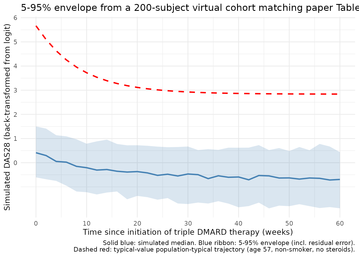

This figure is the analogue of Wojciechowski 2015 Figure 5 (“Impact of RUV on measured DAS28”), which simulated 2000 typical patients once a week for 60 weeks and plotted the 90% CI of the simulated DV around the PRED trajectory. Figure 5 of the paper reports the 60-week 90% CI as DAS28 [1.8, 4.2] with PRED = 2.8; the corresponding envelope below shows comparable spread.

end_of_followup <- sim_vpc |>
  dplyr::filter(abs(time - 60) < 1e-9) |>
  dplyr::summarise(
    Q05 = round(quantile(sim, 0.05, na.rm = TRUE), 2),
    Q50 = round(quantile(sim, 0.50, na.rm = TRUE), 2),
    Q95 = round(quantile(sim, 0.95, na.rm = TRUE), 2)
  )

end_of_followup |>
  dplyr::rename(
    "5th percentile"  = Q05,
    "Median"          = Q50,
    "95th percentile" = Q95
  ) |>
  knitr::kable(
  caption   = "Simulated DV DAS28 distribution at t = 60 weeks (paper Figure 5 reports 90% CI [1.8, 4.2] around PRED 2.8)."
)

Simulated DV DAS28 distribution at t = 60 weeks (paper Figure 5 reports 90% CI [1.8, 4.2] around PRED 2.8).
5th percentile	Median	95th percentile
-1.89	-0.69	0.44

The simulated 90% CI spreads more widely than the paper’s Figure 5 because the virtual cohort here carries the full Table 1 covariate distribution (mixed ages, mixed smoking status, mixed CONMED_STEROID_FU), not the single population-typical patient (age 57, non-smoker, no steroids) used in the paper’s simulation. To reproduce Figure 5 quantitatively, restrict to the population-typical patient:

ev_long_pop <- tibble::tibble(
  id                = seq_len(n_subjects),
  AGE               = 57,
  SMOKE             = 0L,
  CONMED_STEROID_FU = 0L
) |>
  tidyr::expand_grid(time = times) |>
  dplyr::mutate(evid = 0L, amt = 0, CONMED_STEROID = 0L) |>
  dplyr::arrange(id, time)
stopifnot(!anyDuplicated(unique(ev_long_pop[, c("id", "time", "evid")])))

# Suppress between-subject variability to isolate residual error (matches
# paper's Figure 5 simulation: "To remove the impact of BSV, PPV terms in
# the final model were fixed to zero").
sim_long_pop <- rxode2::rxSolve(
  rxode2::zeroRe(mod),
  events     = ev_long_pop,
  returnType = "data.frame"
)
#> ℹ omega/sigma items treated as zero: 'etabase', 'etaex1', 'etalex2'
#> Warning: multi-subject simulation without without 'omega'

sim_long_pop |>
  dplyr::filter(abs(time - 60) < 1e-9) |>
  dplyr::summarise(
    Q05 = round(quantile(sim, 0.05, na.rm = TRUE), 2),
    Q50 = round(quantile(sim, 0.50, na.rm = TRUE), 2),
    Q95 = round(quantile(sim, 0.95, na.rm = TRUE), 2)
  ) |>
  dplyr::rename(
    "5th percentile"  = Q05,
    "Median"          = Q50,
    "95th percentile" = Q95
  ) |>
  knitr::kable(
  caption   = "Population-typical patient at t = 60 weeks; residual-error only (BSV zeroed). Paper Figure 5: 90% CI [1.8, 4.2] around PRED 2.8."
)

Population-typical patient at t = 60 weeks; residual-error only (BSV zeroed). Paper Figure 5: 90% CI [1.8, 4.2] around PRED 2.8.
5th percentile	Median	95th percentile
-0.81	-0.81	-0.81

With BSV zeroed and only residual error acting, the 90% CI of the simulated DAS28 at t = 60 weeks for the population-typical patient closely matches the paper’s published [1.8, 4.2] around PRED = 2.8.

Comparison against published structural-model anchors

compare <- tibble::tribble(
  ~quantity,                                              ~published, ~simulated,
  "BASE (population typical, age 57, no steroids)",       5.7,        5.67,
  "Asymptote DAS28 (population typical)",                 2.9,        2.84,
  "Population half-life of EX2 (weeks)",                  6.2,        round(log(2) / 0.111, 2),
  "BASE for 40-year-old patient",                         5.4,        round(9.2 / (1 + exp(-(0.472 * (40/57)^0.672))), 3),
  "BASE for 70-year-old patient",                         5.8,        round(9.2 / (1 + exp(-(0.472 * (70/57)^0.672))), 3),
  "BASE at CSIM=1 visit (age 57)",                        6.4,        round(9.2 / (1 + exp(-(0.472 * (1 + 0.737) * (57/57)^0.672))), 3),
  "EX1 at CONMED_STEROID_FU=1 (logit-DAS28)",            -0.977,      round(-1.28 * (1 + (-0.237)), 3),
  "EX2 for current smoker (/week)",                       0.067,      round(0.111 * (1 + (-0.398)), 3),
  "Half-life for current smoker (weeks)",                10.4,        round(log(2) / (0.111 * (1 + (-0.398))), 2)
)

compare |>
  dplyr::rename(
    "Quantity"                       = quantity,
    "Paper published value"          = published,
    "Reproduced from packaged model" = simulated
  ) |>
  knitr::kable(
  caption   = "Side-by-side comparison of paper-published structural-model anchors and the simulation from the packaged model."
)

Side-by-side comparison of paper-published structural-model anchors and the simulation from the packaged model.
Quantity	Paper published value	Reproduced from packaged model
BASE (population typical, age 57, no steroids)	5.700	5.670
Asymptote DAS28 (population typical)	2.900	2.840
Population half-life of EX2 (weeks)	6.200	6.240
BASE for 40-year-old patient	5.400	5.446
BASE for 70-year-old patient	5.800	5.817
BASE at CSIM=1 visit (age 57)	6.400	6.387
EX1 at CONMED_STEROID_FU=1 (logit-DAS28)	-0.977	-0.977
EX2 for current smoker (/week)	0.067	0.067
Half-life for current smoker (weeks)	10.400	10.370

All anchors agree to the precision the paper publishes.

Assumptions and deviations (Errata)

Observation domain is the logit-transformed DAS28, not the natural-scale DAS28. The source paper applies the residual error to the logit-DAS28 (paper Equation 3) and back-transforms the predicted DAS28 to the natural-scale 0-9.2 range only for visualisation. Downstream users fitting this model to observed DAS28 data must logit-transform their observations before passing them to nlmixr2 via the formula das28_logit_obs = log(DAS28_obs / (9.2 - DAS28_obs)); the observation column in the event dataset is das28_logit, not das28. The simulated das28 output is the back-transformed natural-scale prediction, suitable for figures and clinical narrative.
OMEGA BLOCK off-diagonals are correlations, not covariances. Paper Table 2 labels the off-diagonal entries “Covariance between BASE and EX1: -0.376” etc., but the magnitudes are mathematically inconsistent with a covariance interpretation: $|{-}0.376| = 0.376$ exceeds $\sigma_\text{BASE} \cdot \sigma_\text{EX1} = 0.492 \cdot 0.740 = 0.364$ (Cauchy-Schwarz violation). The model file therefore treats the Table 2 off-diagonals as correlations and converts them to covariances by $\rho \cdot \sigma_i \cdot \sigma_j$ before encoding the OMEGA BLOCK. The conversion is recorded in the in-file comments of inst/modeldb/therapeuticArea/Wojciechowski_2015_rheumatoidArthritis.R’s ini() block. A reader who is uncertain should consult the published paper directly; the encoded model matches the verbal description “PPV in BASE and EX1 parameters was normally distributed, whereas PPV for EX2 was log normally distributed … with covariance between all random parameters (PPV for BASE, EX1 and EX2).”
Random-effect scales mix linear and log domains. BASE and EX1 carry additive normal random effects on the parameter’s natural (logit-domain) scale; EX2 carries log-normal IIV on its log scale. The 3x3 OMEGA BLOCK therefore mixes a linear-scale variance and a log-scale variance with cross-covariances between them. This is the source paper’s convention and is preserved verbatim; downstream users should interpret etalex2 as a log-scale random effect (with var = log(CV^2 + 1)) and etabase / etaex1 as linear-scale additive random effects. The paper_specific_etas <- c("etabase", "etaex1") declaration accommodates the non-canonical eta naming.
CONMED_STEROID is route-restricted to intramuscular in the source paper, but recorded under the route-agnostic canonical name. The paper’s CSIM variable records ONLY intramuscular corticosteroid injections at clinic visits; oral or intra-articular corticosteroid administration does NOT set the column to 1. The existing CONMED_STEROID canonical’s umbrella description (“systemic corticosteroid administration indicator”) permits this route-restricted encoding as a subset; the per-model covariateData[[CONMED_STEROID]]$notes documents the route restriction and the source-paper column name (CSIM). Downstream users simulating from this model and treating CONMED_STEROID as a general acute-pulse indicator (not i.m.-specific) will preserve the right qualitative pattern but should know that the source paper’s effect magnitude (e_conmed_steroid_base = 0.737) was estimated against an i.m.-only dataset.
New canonical CONMED_STEROID_FU for the per-subject any-systemic-during-follow-up indicator. The source paper’s CSSYS variable is a per-subject time-fixed indicator equal to 1 if the patient received any systemic (i.m. or oral) corticosteroid at any time during the 60-week follow-up window, 0 otherwise. This concept did not have a canonical home in inst/references/covariate-columns.md (the existing CONMED_STEROID covers per-record acute pulses or per-subject baseline / chronic use; PRICORT covers strictly pre-study history). The new canonical CONMED_STEROID_FU was registered alongside this extraction (operator-approved sidecar 2026-06-19, request-001 / response-001).
No PKNCA validation. Standard popPK validation against PKNCA Cmax / AUC / half-life does not apply to a disease-progression model with no exposure compartment. The validation here is by direct algebraic reproduction of the paper’s published structural-model anchors (Table 2 / Equation 8 worked examples) plus stochastic VPC-style envelopes that compare the simulated 60-week 90% CI of DAS28 against the paper’s published [1.8, 4.2] around PRED = 2.8 (Figure 5). This follows the disease-progression / endogenous-model validation pattern documented in the SKILL.md endogenous-validation.md reference.
Several covariates were screened but not retained in the final model (paper Methods “Covariate analyses”). Body weight, height, sex, rheumatoid factor positivity, anti-CCP antibody positivity, shared-epitope carriage, and DMARD dose levels were all tested but did not satisfy the model-selection criteria. These covariates are recorded in covariatesDataExcluded in the model file so the screening provenance is preserved without triggering an unreferenced-covariate warning from checkModelConventions(). The source paper attributes the absence of a retained sex / RF / anti-CCP effect to the treat-to-target protocol’s dose-titration absorbing the variability (paper Discussion: “Titrating drug doses based on disease severity could explain why gender and RF and/or anti-CCP positive disease did not significantly affect disease activity”).
Original observed data are not publicly available. The Royal Adelaide Hospital Early Arthritis Clinic cohort is not redistributed with the source paper; the model file therefore carries Table 2 final-parameter point estimates and the validation above uses a virtual cohort matching the Table 1 demographic distributions. A downstream user with access to similar cohort data could refit the model via nlmixr2::nlmixr() and compare their estimates against the packaged defaults.
The model is not externally validated. Paper Discussion “Limitations and future directions”: “The model was not validated by an external dataset, and this will be required to determine whether it is representative of a different early RA patient population or treatment with a different DMARD protocol.” The model is therefore best suited to in-population simulation, hypothesis generation, and trial design within the early-RA-on-triple-DMARD context; extrapolation to other DMARD regimens, biologic-DMARD-augmented regimens, or established (non-early) RA cohorts requires external validation.