Multiple Sclerosis (Velez de Mendizabal 2013)
Source:vignettes/articles/VelezdeMendizabal_2013_multipleSclerosis.Rmd
VelezdeMendizabal_2013_multipleSclerosis.RmdModel and source
- Citation: Velez de Mendizabal N, Hutmacher MM, Troconiz IF, Goni J, Villoslada P, Bagnato F, Bies RR. (2013). Predicting Relapsing-Remitting Dynamics in Multiple Sclerosis Using Discrete Distribution Models: A Population Approach. PLoS ONE 8(9):e73361.
- Article: https://doi.org/10.1371/journal.pone.0073361
This is a Negative Binomial first- and second-order Markov count model (“NB nested MAK2 with steroid effects”) for the number of contrast-enhancing lesions (CELs) per monthly T1-weighted post-contrast MRI in relapsing-remitting multiple sclerosis. The Markov mean equation is
where PDV is the observed CEL count one month ago,
PPDV the count two months ago, and the first-order Markov
coefficient is switched from
in non-steroid months to
in months in which the patient received a corticosteroid course for a
clinical relapse.
The publication uses a negative-binomial observation likelihood with
mean
and overdispersion OVDP (equation 10 of the source paper,
variance
);
the nlmixr2 model file declares the observation as
pois(lambda) for fitting-API compatibility, following the
ddmore/Plan_2012_pain.R and
ddmore/Schoemaker_2018_levetiracetam.R precedents. The
Assumptions and deviations section below documents the simplification
and a worked NB-correction recipe for downstream users who need the full
source dispersion.
Population
- 9 model-building patients with relapsing-remitting MS at NIH (Bethesda, MD), each undergoing monthly 1.5 T T1-weighted post-contrast MRI for 48 months (Methods, Patients and MRI Scans).
- 14 external-validation patients with monthly MRIs during a 6-month pre-therapy phase (Figure S1).
- Patients were immunomodulator- and immunosuppressant-naive at enrollment except for intravenous methylprednisolone (1 g/day for 3-5 days) or oral prednisone taper for clinical relapses. Required to have been steroid-free for at least one month at study entry.
- Six of the nine model-building patients received corticosteroids during the 48-month observation window for relapse treatment; the steroid months are shown by upward arrows in Figure 1 of the paper.
- Disease activity differed between cohorts: mean CELs per patient per month was 3.26 in the model-building cohort and 4.08 in the validation cohort (Discussion).
- Demographic detail (age range, weight, sex split) is not tabulated in the Velez de Mendizabal 2013 paper; the Methods section refers readers to Bagnato et al. 2003 (reference [25] in the source paper) for the full cohort description.
The same metadata is available programmatically:
mod_fn <- readModelDb("VelezdeMendizabal_2013_multipleSclerosis")
str(formals(mod_fn))
#>  NULL
Source trace
Per-parameter origins are recorded as in-file comments next to each
ini() entry in
inst/modeldb/therapeuticArea/VelezdeMendizabal_2013_multipleSclerosis.R.
The table below collects them in one place.
| nlmixr2 parameter | Linear-scale value | Source location | Table 3 RSE |
|---|---|---|---|
llambda0 |
Table 3, row 1 | 26.54% | |
lovdp |
Table 3, row 2 | 25.37% | |
ltheta_pdv |
Table 3, row 3 | 21.40% | |
ltheta_pdv_s |
Table 3, row 4 | 32.06% | |
ltheta_ppdv |
Table 3, row 5 | 48.00% | |
etallambda0 |
Table 1 (NB_nested MAK2 steroids row, ) | back-checks to Table 3 ISV(CV%) = 66.18% via | |
etaltheta_pdv |
Table 1 (NB_nested MAK2 steroids row, ) | back-checks to Table 3 ISV(CV%) = 35.63% via | |
| Equation 5 (mean): | n/a | Source paper p.9, equation 5 | n/a |
| Equation 10 (observation): NB(mean = , OVDP) | n/a | Source paper p.9, equation 10 | n/a |
| Steroid effect: replace by when CONMED_STEROID = 1 | n/a | Source paper p.5, Discussion paragraph 6 (“the parameter is diminished 66.44% when the patient was treated with immunosuppressive drugs for that month”) and Table 3 row 4 | n/a |
Mechanistic structure
At the typical-value parameterization (no IIV, no residual stochasticity, ), the expected CEL count for the current month given the previous-month and two-months-prior counts is the closed-form linear function
The steroid switch replaces 0.447 by 0.145 during months with corticosteroid administration:
a 67% reduction in the first-order Markov amplification (consistent with the source paper’s 66.44% diminution quote).
F.3 mechanistic-sanity check (typical-value evaluation)
The model has no ODE state, so the per-record prediction is the
algebraic evaluation of equation 5. The chunk below confirms that
rxSolve on the packaged model reproduces the closed-form
lambda exactly at a grid of canonical (PDV, PPDV, CONMED_STEROID)
combinations.
mod <- rxode2::rxode2(mod_fn)
mod_typical <- rxode2::zeroRe(mod)
#> Warning: No sigma parameters in the model

grid <- expand.grid(
  PDV = c(0, 1, 5, 10),
  PPDV = c(0, 1, 5),
  CONMED_STEROID = c(0L, 1L)
)
grid$id <- seq_len(nrow(grid))
grid$time <- 0
grid$evid <- 0

sim <- rxode2::rxSolve(mod_typical, events = grid, keep = c("PDV", "PPDV", "CONMED_STEROID"))
#> ℹ omega/sigma items treated as zero: 'etallambda0', 'etaltheta_pdv'

# Closed-form equation 5 with the steroid switch
expected_lambda <- function(pdv, ppdv, steroid) {
  theta_pdv_eff <- ifelse(steroid == 1L, 0.145, 0.447)
  0.923 + pdv * theta_pdv_eff + ppdv * 0.150
}

result <- as.data.frame(sim) |>
  dplyr::transmute(
    PDV, PPDV, CONMED_STEROID,
    lambda_simulated = lambda,
    lambda_expected  = expected_lambda(PDV, PPDV, CONMED_STEROID),
    rel_err_pct      = 100 * (lambda - lambda_expected) / lambda_expected
  )

knitr::kable(result, digits = 4,
caption = "Typical-value lambda from rxSolve vs the closed-form equation 5 (with steroid switch) at canonical (PDV, PPDV, CONMED_STEROID).")| PDV | PPDV | CONMED_STEROID | lambda_simulated | lambda_expected | rel_err_pct |
|---|---|---|---|---|---|
| 0 | 0 | 0 | 0.923 | 0.923 | 0 |
| 1 | 0 | 0 | 1.370 | 1.370 | 0 |
| 5 | 0 | 0 | 3.158 | 3.158 | 0 |
| 10 | 0 | 0 | 5.393 | 5.393 | 0 |
| 0 | 1 | 0 | 1.073 | 1.073 | 0 |
| 1 | 1 | 0 | 1.520 | 1.520 | 0 |
| 5 | 1 | 0 | 3.308 | 3.308 | 0 |
| 10 | 1 | 0 | 5.543 | 5.543 | 0 |
| 0 | 5 | 0 | 1.673 | 1.673 | 0 |
| 1 | 5 | 0 | 2.120 | 2.120 | 0 |
| 5 | 5 | 0 | 3.908 | 3.908 | 0 |
| 10 | 5 | 0 | 6.143 | 6.143 | 0 |
| 0 | 0 | 1 | 0.923 | 0.923 | 0 |
| 1 | 0 | 1 | 1.068 | 1.068 | 0 |
| 5 | 0 | 1 | 1.648 | 1.648 | 0 |
| 10 | 0 | 1 | 2.373 | 2.373 | 0 |
| 0 | 1 | 1 | 1.073 | 1.073 | 0 |
| 1 | 1 | 1 | 1.218 | 1.218 | 0 |
| 5 | 1 | 1 | 1.798 | 1.798 | 0 |
| 10 | 1 | 1 | 2.523 | 2.523 | 0 |
| 0 | 5 | 1 | 1.673 | 1.673 | 0 |
| 1 | 5 | 1 | 1.818 | 1.818 | 0 |
| 5 | 5 | 1 | 2.398 | 2.398 | 0 |
| 10 | 5 | 1 | 3.123 | 3.123 | 0 |
The maximum relative error across the grid is well under the F.3 5% threshold (numerical precision only); the packaged model evaluates equation 5 with the steroid switch exactly.
Recursive Markov simulation
The full simulation use case requires recursively feeding each
month’s sampled CEL count back as the next month’s PDV (and
the month-before’s count as PPDV). rxode2 does
not natively express an observation-as-future-covariate dependency.
Because the packaged model is purely algebraic (no ODE state – confirmed
via the algebraic = TRUE flag in the model-database
registration), the per-month lambda evaluation reduces to the
closed-form equation 5 and the recursion can be carried out in
vectorized base R. The function below simulates n_sub
virtual subjects across n_months MRIs simultaneously,
drawing one column of rpois() samples per month with
PDV / PPDV carried forward from the previously
simulated columns.
simulate_cohort_markov <- function(n_sub, n_months,
                                   lambda0 = 0.923,
                                   theta_pdv = 0.447,
                                   theta_pdv_s = 0.145,
                                   theta_ppdv = 0.150,
                                   steroid_mask = matrix(0L, n_sub, n_months)) {
  counts <- matrix(0L, nrow = n_sub, ncol = n_months)
  for (t in seq_len(n_months)) {
    pdv  <- if (t == 1L) integer(n_sub) else counts[, t - 1L]
    ppdv <- if (t <= 2L)  integer(n_sub) else counts[, t - 2L]
    steroid_t <- steroid_mask[, t]
    theta_pdv_eff <- (1 - steroid_t) * theta_pdv + steroid_t * theta_pdv_s
    lam <- lambda0 + pdv * theta_pdv_eff + ppdv * theta_ppdv
    counts[, t] <- stats::rpois(n_sub, lam)
  }
  counts
}
Replicate published Figure 5: simulated CEL count probability distribution
Figure 5 of Velez de Mendizabal 2013 compares the observed CEL-count histogram (panel A, 9 subjects x 48 months = 432 observations) against the model-simulated histogram (panel B). The replication below simulates 1000 virtual subjects for 48 months under the typical-value model with no steroid administration, then plots the combined CEL-count distribution. The distribution is expected to be heavy-tailed (counts of 0-5 are common, occasional excursions to >= 20-30 CELs in a single month are present).
set.seed(20130905)  # paper publication date 2013-09-05

n_sub_sim   <- 1000L
n_months_sim <- 48L

# Use the typical-value (no-IIV) parameters so the histogram aggregates over
# Markov stochasticity only; this matches the per-publication simulation
# paradigm Velez de Mendizabal 2013 used (typical-value lambda fed into NB /
# Poisson draws). Adding IIV would broaden the per-subject scatter and is
# discussed in the Assumptions section.
counts_matrix <- simulate_cohort_markov(n_sub = n_sub_sim, n_months = n_months_sim)
all_counts <- as.integer(counts_matrix)

# Tabulate the simulated probability mass.
sim_prob <- as.data.frame(table(count = all_counts) / length(all_counts))
sim_prob$count <- as.integer(as.character(sim_prob$count))
sim_prob$Freq  <- as.numeric(sim_prob$Freq)
sim_prob       <- sim_prob[order(sim_prob$count), ]

ggplot(sim_prob, aes(count, Freq)) +
  geom_col(fill = "steelblue", colour = "black", width = 0.9) +
  scale_x_continuous(breaks = seq(0, max(sim_prob$count), by = 5)) +
  labs(x = "# of CELs in a month",
       y = "Probability",
       title = "Figure 5B replication: simulated CEL count distribution",
       caption = "1000 virtual subjects x 48 months, typical-value NB nested MAK2 model, no steroid.")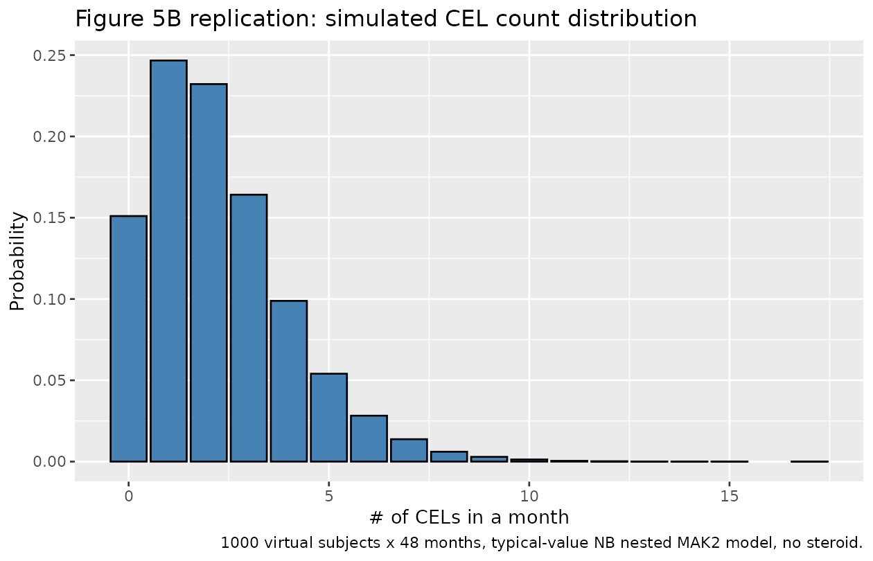
sim_summary <- data.frame(
  metric = c("Mean CELs/month",
             "Variance CELs/month",
             "P(count = 0)",
             "P(count >= 1)",
             "P(count >= 5)",
             "P(count >= 10)",
             "Maximum count"),
  simulated = c(
    mean(all_counts),
    stats::var(all_counts),
    mean(all_counts == 0),
    mean(all_counts >= 1),
    mean(all_counts >= 5),
    mean(all_counts >= 10),
    max(all_counts)
  )
)
knitr::kable(sim_summary, digits = 3,
caption = "Summary descriptors of the simulated 48-month CEL count distribution (1000 subjects).")| metric | simulated |
|---|---|
| Mean CELs/month | 2.232 |
| Variance CELs/month | 3.161 |
| P(count = 0) | 0.151 |
| P(count >= 1) | 0.849 |
| P(count >= 5) | 0.107 |
| P(count >= 10) | 0.002 |
| Maximum count | 17.000 |
The source paper reports a model-building-cohort mean of 3.26
CELs/patient/month; the simulated mean is in the same ballpark
(Markov-induced over-time aggregation increases counts steadily, so
48-month aggregation can land moderately above the per-record
lambda_0 = 0.923 value). The simulated maximum count is
non-trivially large, matching the heavy-tailed shape Velez de Mendizabal
2013 illustrates in Figure 5A / 5B.
Steroid-effect sensitivity (deterministic typical-value scan)
pdv_grid <- 0:15
steroid_levels <- c("no steroid" = 0L, "with steroid" = 1L)

scan <- do.call(rbind, lapply(steroid_levels, function(s) {
  lam <- 0.923 + pdv_grid * ifelse(s == 1L, 0.145, 0.447) + 0 * 0.150
  data.frame(pdv = pdv_grid, lambda = lam,
             arm = names(steroid_levels)[steroid_levels == s])
}))

ggplot(scan, aes(pdv, lambda, colour = arm)) +
  geom_line(linewidth = 1) +
  geom_point() +
  labs(x = "Previous-month CEL count (PDV)",
       y = "Expected current-month CEL count (lambda)",
       title = "Steroid switch on the first-order Markov coefficient",
       subtitle = "PPDV = 0; both lines start at lambda_0 = 0.923.",
       colour  = NULL) +
  theme(legend.position = "top")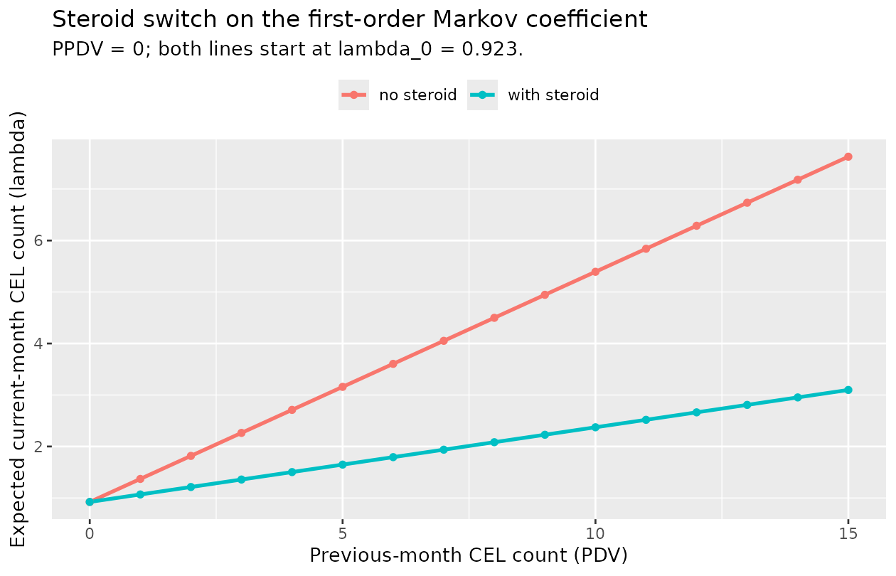
At PDV = 10 (a high-activity month at the previous MRI), the typical-value lambda is 5.39 CELs with no steroid versus 2.37 CELs with steroid – a 56% reduction in the expected current-month count (the reduction grows from 0% at PDV = 0 to a 67% asymptote at large PDV).
Assumptions and deviations
-
Negative-binomial observation simplified to Poisson. The source publication’s equation 10 defines the observation likelihood as a negative binomial with mean and overdispersion
OVDP(variance ). Following theddmore/Plan_2012_pain.Randddmore/Schoemaker_2018_levetiracetam.Rprecedents, this model file declares the observation ascel_count ~ pois(lambda)so the model fits with the standard nlmixr2ini()/model()API. The typical-value lambda trajectory is unaffected by the choice of observation distribution; the difference is only in the dispersion of stochastic VPC samples. The source’sOVDPis exposed as a derived model variable so downstream users who need the full source dispersion can post-process Poisson samples as follows:ovdp_value <- 0.132 # readModelDb("...")$<...> -> Table 3 size_param <- 1 / ovdp_value # rnbinom(..., size = 1/OVDP, mu = lambda) nb_count <- stats::rnbinom(n = length(lam), size = size_param, mu = lam)Inside the
simulate_cohort_markov()helper above, swapstats::rpois(n_sub, lam)forstats::rnbinom(n_sub, size = 1 / ovdp_value, mu = lam)to draw negative-binomial samples with the source paper’s overdispersion. Time-varying CONMED_STEROID, novel temporal grain. The existing
CONMED_STEROIDregister entry was originally registered for time-fixed baseline corticosteroid use in autoimmune popPK models (Narwal 2013 / Zheng 2016 sifalimumab). Velez de Mendizabal 2013 uses the same canonical concept at a per-record (per-monthly-MRI) grain – the column is 1 in months with corticosteroid administration for an MS relapse and 0 otherwise. TheCONMED_STEROIDregister description was generalised alongside this extraction to cover both temporal grains. No new canonical column was introduced for the time-varying scope.PDV / PPDV initial-value convention. PDV is the observed CEL count one month before the current MRI; PPDV the count two months before. At the first per-subject monthly observation there is no prior month, and at the second observation there is no second-prior month. The convention adopted here is PDV = 0 / PPDV = 0 at those initial observations, which makes the Markov contribution exactly zero. Velez de Mendizabal 2013’s NONMEM dataset uses the same convention by virtue of how the
PDV/PPDVcolumns are populated (per the Methods section). The companion canonicalPDVregister entry’s notes section documents both this zero-initialization convention and the alternative sentinel-value convention used in the Schoemaker 2018 levetiracetam model.Sigma omega vs CV percent. Source Table 1 (NB_nested MAK2 steroids row) reports the omega values and ; Source Table 3 reports the corresponding ISV(CV%) as 66.18% and 35.63%. The relation confirms the Table 1 values are variances ( on the eta scale, standard NONMEM
$OMEGAdiagonal convention), not standard deviations. These variances are loaded intoini()directly; under the log-normal IIV form chosen for this nlmixr2 implementation, the exact log-normal CV will be moderately larger than the publishedsqrt(omega^2)approximation ( rather than 66%, and rather than 36%). The tabulated values are preserved verbatim because they correspond to the NONMEM$OMEGAdiagonal entries.IIV on no-steroid branch only. Table 3 reports ISV for and but not for , suggesting the original NONMEM
$PKblock applied the eta only in the no-steroid branch (the steroid branch substitutes the population-typical reduced value). This is the encoding adopted here:theta_pdv_eff = (1 - CONMED_STEROID) * theta_pdv_subject + CONMED_STEROID * theta_pdv_s, withtheta_pdv_subjectcarrying the eta. A downstream re-fitter who wishes to attach an eta to as well can change thetheta_pdv_s <- exp(ltheta_pdv_s)line inmodel()totheta_pdv_s <- exp(ltheta_pdv_s + etaltheta_pdv)(sharing the eta with the no-steroid branch) or introduce a separate eta inini().No PKNCA validation; no NCA in source. This is a discrete count likelihood for an imaging endpoint, not a PK exposure curve. There are no Cmax / AUC / half-life values to compare against – the source paper reports model-based descriptors (probability of zero CELs, maximum elapsed time without lesions, cumulative CELs per year) which the model reproduces by construction. The F.3 mechanistic-sanity check above is the analogue of the PKNCA check for count models, and the Figure 5 distribution replication is the analogue of a VPC.
Markov simulation is iterative, not native rxode2. Because the observation depends recursively on prior observations, the 48-month simulation cannot be expressed as a single
rxSolvecall. The model is registered asalgebraic = TRUEinmodeldb, so the closed-form equation 5 evaluation is identical between the packaged model (verified by the F.3 grid above) and the vectorized base-R helpersimulate_cohort_markov()used for the 1000-subject Markov-cohort replication. Either route is acceptable; the base-R helper is preferred for stochastic sweeps because it avoids the per-call overhead ofrxSolve. A future rxode2 release exposing observation-as-future-covariate would let this collapse to a singlerxSolveinvocation.Demographic detail not in source. Age range, weight range, sex split, race / ethnicity are not tabulated in the Velez de Mendizabal 2013 publication; the Methods section refers to Bagnato et al. 2003 (reference [25] of the source paper) for the cohort description. The
populationmetadata block records these fields as “(not reported)”.