Joint tumor-size / overall-survival framework in NSCLC (Struemper 2025)
Source:vignettes/articles/Struemper_2025_tumorsize_OS_nsclc.Rmd
Struemper_2025_tumorsize_OS_nsclc.RmdModel and source
- Citation: Struemper H, Rathi C, Muliaditan M, Goulooze SC, Franzese RC, Mantero A, Melhem M, Post TM, Visser SAG. Development of a Joint Tumor Size-Overall Survival Modeling and Simulation Framework Supporting Oncology Development Decision-Making. CPT Pharmacometrics Syst Pharmacol. 2025;14(6):1006-1017. doi:10.1002/psp4.70002. PMID: 39985158.
- Description: Joint tumor-size (TS) / overall-survival (OS) framework model for non-small cell lung cancer (NSCLC), developed by Struemper et al. (GSK) on pooled individual-level data from 786 participants across seven GSK-sponsored clinical trials (INDUCE-1, INDUCE-2, Entree Lung Part 2, GARNET, AMBER, INTR@PID LUNG 037, PERLA) spanning immunotherapy, chemotherapy, and combinations thereof. The TS sub-model is the bi-exponential Stein model with per-treatment-arm typical tumor-growth (kge) and tumor-shrinkage (kse) rates selected at simulation / fit time via the TRT categorical covariate (12 levels; see covariateData[[TRT]] for the integer coding). The OS sub-model is an accelerated failure time (AFT) log-normal survival with a treatment-agnostic link to individual TS parameters: tumor growth rate kge enters via a fixed Emax function, baseline TS and time-to-tumor-growth (TTG) enter linearly, and three baseline laboratory covariates (albumin, total protein, neutrophil-to-lymphocyte ratio) are additive on the log-time scale. TS is observed in mm (sum of longest diameters of target lesions per RECIST 1.1); survival is reported on the day scale in the source paper and converted to weeks inside model() so the entire model runs on a single weeks time axis.
- Article: CPT Pharmacometrics Syst Pharmacol. 2025;14(6):1006-1017
- Supplement: Data S1 (Tables S1-S3, Figures S1-S4)
This is a joint tumor-size (TS) / overall-survival (OS)
framework model, not a drug-specific PK/PD model: a
single multi-treatment-arm Stein bi-exponential TS sub-model is coupled
to an accelerated failure-time (AFT) log-normal survival sub-model whose
covariates are the individual TS parameters plus three baseline
laboratory values. The model was fit jointly to individual-level data
from 786 participants across seven GSK-sponsored NSCLC trials. The
packaged model in
inst/modeldb/therapeuticArea/oncology/Struemper_2025_tumorsize_OS_nsclc.R
ships per-arm typical-value tumor growth (kge) and
shrinkage (kse) rate constants for all 12 treatment
categories; the active arm is selected at simulation / fit time by the
TRT categorical covariate (1-12 integer coding documented
in mod$covariateData$TRT$notes).
Population
The pooled cohort is 786 adults with advanced or metastatic NSCLC across seven GSK-sponsored trials (INDUCE-1, INDUCE-2, Entree Lung Part 2, GARNET, AMBER, INTR@PID LUNG 037, PERLA; Struemper 2025 Table 1). Median OS follow-up was 277 days and 430 OS events were observed across 3,702 TS observations. The treatment landscape spans immunotherapy (anti-PD-1 / anti-PD-L1 / anti-LAG-3 / anti-TIM-3 / anti-CTLA-4 / anti-ICOS / anti-OX40), chemotherapy, and combinations.
The reference-subject baseline covariates the source paper uses for Figure 3 (the typical-subject covariate values that the model’s centring constants are tied to) are:
| Covariate | Reference value | Source |
|---|---|---|
LDH baseline lactate dehydrogenase |
225.5 IU/L | Figure 3 caption |
PDL1_TUM tumor PD-L1 expression (PD-1 inhibitor arms
only) |
15 % | Figure 3 caption |
| baseline number of target lesions | 2 (population median); model equation centres at 3 | Figure 3 caption |
TSb baseline tumor size |
74 mm (population median); TVTSb = 86.07
mm at NTARGET = 3
|
Figure 3 caption |
kge tumor growth rate |
0.013 1/week (illustrative) | Figure 3 caption |
TTG time to tumor growth |
14 weeks (illustrative) | Figure 3 caption |
ALB baseline albumin |
39.4 g/L | Figure 3 caption |
TPRO baseline total protein |
71 g/L | Figure 3 caption |
NLR baseline neutrophil-to-lymphocyte ratio |
4.1 | Figure 3 caption |
The same metadata is available programmatically:
str(readModelDb("Struemper_2025_tumorsize_OS_nsclc")()$population)
#> ℹ Joint TS-OS framework model for advanced/metastatic NSCLC (Struemper 2025, n=786, 7 GSK trials). TS = Stein bi-exponential with per-treatment-arm kge/kse (selected by TRT integer 1-12); OS = AFT log-normal with treatment-agnostic link (kge Emax + TSb + TTG linear) plus baseline ALB, TPRO, NLR. Outputs: TS (observable, mm), mu_os_logwks, sigma_os, sur (S(t)), hazard. PDL1_TUM effect on kse is gated by a derived has_pd1 indicator (1 if TRT == 1 or TRT >= 6, else 0). NTARGET (count) is binarised to NTARGET_GE3 per the library's count-covariate policy; Box-Cox IIV on kge (paper shape -0.3744) is omitted in favour of standard log-normal IIV. Both deviations are documented in the vignette Errata.
#> List of 10
#>  $ species       : chr "human (adults with advanced/metastatic NSCLC)"
#>  $ n_subjects    : int 786
#>  $ n_studies     : int 7
#>  $ age_range     : chr "not reported in this paper; advanced/metastatic NSCLC trial cohorts"
#>  $ sex_female_pct: num NA
#>  $ race_ethnicity: chr "not reported in this paper at the pooled level (per-study demographics are in the underlying trial publications)"
#>  $ disease_state : chr "advanced/metastatic NSCLC (locally advanced, Stage IIIb/IIIc, Stage IV, recurrent, or metastatic per each study"| __truncated__
#>  $ dose_range    : chr "n/a (no PK input; per-arm dosing was the protocol-defined dose per study)"
#>  $ regions       : chr "multiregional across seven clinical trials (per-study geographic mix not pooled in this paper)"
#>  $ notes         : chr "Pooled-cohort baseline covariate medians (Struemper 2025 Figure 3 caption; population-typical reference values "| __truncated__
The per-arm subject counts and per-arm TVKG / TVKS estimates are
encoded inline as lkge_<arm> and
lkse_<arm> ini() parameters and selected
at run time by TRT (see Source trace below for the full
register).
Source trace
The per-parameter origin is also recorded as an in-file comment next
to each ini() entry in
inst/modeldb/therapeuticArea/oncology/Struemper_2025_tumorsize_OS_nsclc.R.
| Quantity | Value | Source |
|---|---|---|
TVTSb baseline tumor size (mm) |
86.07 | Table 2 |
TVKG PEMBRO (1/week) |
0.00651 | Table 2 |
TVKG FELAD (1/week) |
0.01135 | Table 2 |
TVKG CHEMO (1/week) |
0.01822 | Table 2 |
TVKG FELAD+CHEMO (1/week) |
0.01672 | Table 2 |
TVKG IO-COMBO (1/week) |
0.01442 | Table 2 |
TVKG DOSTAR (1/week) |
0.008105 | Table 2 |
TVKG DOSTAR+CHEMO (1/week) |
0.008845 | Table 2 |
TVKG PEMBRO+CHEMO (1/week) |
0.01153 | Table 2 |
TVKG COBO100MG+DOSTAR cohort B (1/week) |
0.01372 | Table 2 |
TVKG COBO300MG+DOSTAR cohort B (1/week) |
0.01257 | Table 2 |
TVKG COBO900MG+DOSTAR cohort B (1/week) |
0.01603 | Table 2 |
TVKG COBO300MG+DOSTAR cohort D (1/week) |
0.01267 | Table 2 |
TVKS PEMBRO (1/week) |
0.01700 | Table 2 |
TVKS FELAD (1/week) |
3.396e-06 (poorly identified) | Table 2 |
TVKS CHEMO (1/week) |
0.03566 | Table 2 |
TVKS FELAD+CHEMO (1/week) |
0.02805 | Table 2 |
TVKS IO-COMBO (1/week) |
0.007894 | Table 2 |
TVKS DOSTAR (1/week) |
0.01615 | Table 2 |
TVKS DOSTAR+CHEMO (1/week) |
0.03504 | Table 2 |
TVKS PEMBRO+CHEMO (1/week) |
0.03499 | Table 2 |
TVKS COBO100MG+DOSTAR cohort B (1/week) |
0.005006 | Table 2 |
TVKS COBO300MG+DOSTAR cohort B (1/week) |
0.01125 | Table 2 |
TVKS COBO900MG+DOSTAR cohort B (1/week) |
0.006273 | Table 2 |
TVKS COBO300MG+DOSTAR cohort D (1/week) |
0.00448 | Table 2 |
| NTARGET effect on TSb (per lesion) | 0.288 | Table 3 footnote a |
PD-L1 effect on kse (per percent) |
0.00902 | Table 3 footnote b |
LDH power exponent on kge
|
0.474 (reference 225.5 IU/L) | Table 3 footnote c |
mu_OS,int intercept (log-days) |
6.94 | Table 3 |
sigma_OS log standard deviation of log-survival |
-0.331 | Table 3 |
Emax of kg on mu_OS
|
-6.91 (FIX) | Table 3 footnote d |
EC50 of kg on mu_OS (1/week) |
0.109 | Table 3 footnote d |
TSb on mu_OS (per mm, centred at 100) |
-0.00366 | Table 3 footnote e |
TTG on mu_OS (per week, centred at 39.9) |
0.0124 | Table 3 footnote f |
ALB on mu_OS (per g/L, centred at 39.4) |
0.0452 | Table 3 footnote g |
TPRO on mu_OS (per g/L, centred at 71) |
0.0194 | Table 3 footnote h |
NLR on mu_OS (per ratio, centred at 4.1) |
-0.0141 | Table 3 footnote i |
| omega^2 TSb | 0.2645 | Table 2 |
| omega^2 kge | 0.8715 | Table 2 |
| omega^2 kse | 0.9174 | Table 2 |
| omega_xy (TSb x kge) | 0.01911 | Table 2 |
| omega_xy (TSb x kse) | -0.06367 | Table 2 |
| omega_xy (kge x kse) | 0.1504 | Table 2 (typeset as ‘KG x KG’ in the PDF; treated as kge x kse in the correlated 3x3 block) |
| sigma^2 additive (mm^2) | 6.324 | Table 2 |
| sigma^2 proportional (fraction^2) | 0.01276 | Table 2 |
| TS Eq. 1 Stein bi-exponential | n/a | Methods Eq. 1 (Stein 2008 [25]) |
| OS Eq. 2 log-normal AFT hazard | n/a | Methods Eq. 2 |
mu_OS link summation |
n/a | Table 3 footnote j |
TTG derived formula (log(ks)-log(kg))/(kg+ks), clipped
at 0 |
n/a | Table S2 |
Mechanism in one paragraph
The Stein bi-exponential TS model
TS(t) = TSb * (exp(kge*t) + exp(-kse*t) - 1) captures the
two dominant features of an oncology TS trajectory: an exponential
growth component governed by kge and a treatment-driven
exponential shrinkage component governed by kse. The
library encodes this as two parallel ODE compartments
growth and shrink with per-subject initial
conditions both equal to TSb, so that
growth(t)+shrink(t)-TSb is algebraically identical to the
Stein closed form and reduces to TSb at t = 0.
Each treatment arm has its own typical kge and
kse; baseline covariates modulate the individual values:
LDH scales kge via a power law
(LDH/225.5)^0.474, PDL1_TUM scales kse
exponentially exp(0.00902 * PDL1_TUM) only for PD-1
inhibitor-containing arms, and the binary NTARGET_GE3
indicator shifts TSb by +28.8 %. The OS sub-model uses an
AFT log-normal distribution with location mu_OS. The
location is constructed from six additive contributions: a
treatment-agnostic Emax effect of individual kge (the
strongest single predictor), a linear effect of individual
TSb, a linear effect of derived TTG (time to tumor growth,
clipped at 0), and three baseline laboratory covariates (ALB, TPRO,
NLR). Crucially the treatment label does not enter
mu_OS directly: every treatment effect on OS flows through
the treatment-specific TS dynamics that drive kge, TSb, and
TTG.
Dimensional check
| Term | Units |
|---|---|
kge * growth |
(1/week) * (mm) = mm / week |
kse * shrink |
(1/week) * (mm) = mm / week |
(LDH/225.5)^0.474 |
unitless |
exp(PDL1_TUM * 0.00902 * has_pd1) |
unitless (0.00902 has units 1/percent) |
1 + 0.288 * NTARGET_GE3 |
unitless |
emax_kge * kge / (kge + ec50_kge) |
unitless (paper coefficient -6.91 on log time) |
mu_os_logdays - log(7) |
log(weeks) |
(log(t_weeks) - mu_os_logwks) / sigma_os |
unitless (standard normal argument) |
pdf_lt / sur |
1 / week (hazard rate on weeks axis) |
All ODE right-hand sides match their state’s
[state]/week requirement and the OS hazard returns 1/week
with t in weeks.
Virtual cohort: representative treatment arms
The full paper analysis includes 12 treatment categories. To keep
this vignette under the pkgdown wall-clock budget, we simulate a 5-arm
sub-panel that spans the main mechanism classes: pembrolizumab
monotherapy (TRT = 1, the canonical default and largest
PD-1 cohort), feladilimab monotherapy (TRT = 2, an
anti-ICOS therapy whose kse is essentially zero so the
Stein model collapses to monotonic growth), docetaxel chemotherapy
(TRT = 3), dostarlimab + chemotherapy
(TRT = 7, a PD-1 + chemo combination), and pembrolizumab +
chemotherapy (TRT = 8, a second PD-1 + chemo combination).
All 12 arms are reachable by passing the corresponding TRT
integer in the event table; no parameter override is required.
We use a baseline-covariate distribution loosely mirroring the
Struemper 2025 pooled cohort (Table S3): NTARGET_GE3 ~ 25 % (since the
population median NTARGET = 2), LDH log-normal centred at 225 IU/L (CV
40 %), ALB normal centred at 39.4 g/L (SD 4), TPRO normal centred at 71
g/L (SD 5), NLR log-normal centred at 4.1 (CV 50 %). For PD-1 inhibitor
arms we draw PDL1_TUM uniformly on [0, 100] %; for non-PD-1 arms
PDL1_TUM is set to 0 (the effect is gated by has_pd1 inside
the model and the value is ignored).
n_per_arm <- 80L

make_cohort <- function(n, trt_code, id_offset, has_pdl1 = TRUE) {
  pdl1 <- if (has_pdl1) runif(n, 0, 100) else rep(0, n)
  tibble(
    id          = id_offset + seq_len(n),
    TRT         = trt_code,
    NTARGET_GE3 = as.integer(rbinom(n, 1, 0.25)),
    LDH         = exp(rnorm(n, log(225), 0.4)),
    PDL1_TUM    = pdl1,
    ALB         = pmax(15, rnorm(n, 39.4, 4)),
    TPRO        = pmax(40, rnorm(n, 71, 5)),
    NLR         = pmin(100, exp(rnorm(n, log(4.1), 0.5)))
  )
}

arms <- tibble::tribble(
  ~label,             ~trt,  ~has_pdl1,
  "PEMBRO",              1L,  TRUE,
  "FELAD",               2L,  FALSE,
  "CHEMO",               3L,  FALSE,
  "DOSTAR+CHEMO",        7L,  TRUE,
  "PEMBRO+CHEMO",        8L,  TRUE
)

cohorts <- arms |>
  mutate(id_offset = (row_number() - 1L) * n_per_arm) |>
  rowwise() |>
  do(make_cohort(n_per_arm, .$trt, .$id_offset, .$has_pdl1) |>
       mutate(arm = .$label)) |>
  ungroup()
The event grid samples TS every 6 weeks out to 78 weeks (1.5 years), matching the typical RECIST scan cadence:
TS trajectories by treatment arm (replicates Figure 3 / Figure S3 qualitative trends)
Figure S3 of the source paper boxplots the per-subject estimated TS
parameters (TSb, kge, kse)
stratified by treatment category; Figure 3 of the source paper shows how
covariate variation translates to TS-parameter percent change. We
replicate the qualitative TS-shape differentiation between the five
representative arms by simulating each cohort with the packaged model
and plotting the mean and IQR of TS over time:
sim <- rxode2::rxSolve(
  mod, events,
  keep = c("arm", "TRT", "NTARGET_GE3", "LDH", "PDL1_TUM", "ALB", "TPRO", "NLR"),
  returnType = "data.frame"
) |>
  filter(time > 0 | time == 0)  # keep t = 0
ts_summary <- sim |>
  group_by(arm, time) |>
  summarise(
    ts_mean = mean(TS),
    ts_q25  = stats::quantile(TS, 0.25),
    ts_q75  = stats::quantile(TS, 0.75),
    .groups = "drop"
  ) |>
  mutate(arm = factor(arm, levels = arms$label))

ggplot(ts_summary, aes(time, ts_mean, fill = arm, color = arm)) +
  geom_ribbon(aes(ymin = ts_q25, ymax = ts_q75), alpha = 0.2, color = NA) +
  geom_line(linewidth = 0.8) +
  labs(
    x = "Weeks since baseline scan",
    y = "Tumor size (mm; sum of longest diameters)",
    caption = "n = 80 simulated subjects per arm. Solid = mean, ribbon = IQR. Algebraic Stein: TS = growth + shrink - TSb."
  ) +
  theme_bw() +
  theme(legend.position = "right")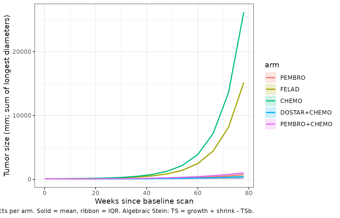
Simulated TS trajectories for five representative treatment arms (n = 80 per arm). Solid line = arm-wise mean of TS(t); ribbon = 25th-75th percentile of the per-subject TS distribution. Qualitative shape mirrors Struemper 2025 Figure S3: arm-specific Stein parameters determine whether TS shrinks, grows, or follows a shrink-then-regrowth pattern.
Three illustrative TS profiles (replicates Figure 4)
Figure 4 of the source paper illustrates that the OS link depends on
both kge (long-time growth) and kse (early
shrinkage) by showing three hand-picked profiles with the same or
different kge / kse combinations. We reproduce
that figure with three named profiles matched to the paper’s Figure 4
captions: red kge=0.01, kse=0.01, blue
kge=0.02, kse=0.10, green kge=0.01, kse=0.10.
The treatment-arm scaffolding is bypassed (since the figure varies
kge and kse directly, not by arm); we pass the
parameters via params= to rxSolve.
mod_typical <- mod |> rxode2::zeroRe()

ev_typ <- rxode2::et(seq(0, 78, by = 1)) |>
  rxode2::as.et()

# Force the typical-subject baseline covariates for the OS link.
typ_one <- function(label, kg_val, ks_val) {
  ev <- as.data.frame(ev_typ)
  ev$evid <- 0L
  ev$amt  <- NA_real_
  ev$cmt  <- "growth"
  ev$TRT  <- 1L
  ev$NTARGET_GE3 <- 0L
  ev$LDH      <- 225.5
  ev$PDL1_TUM <- 0   # remove the PDL1 effect on ks so the override sticks
  ev$ALB      <- 39.4
  ev$TPRO     <- 71
  ev$NLR      <- 4.1
  s <- rxode2::rxSolve(
    mod_typical, ev,
    params = c(lkge_pembro = log(kg_val), lkse_pembro = log(ks_val)),
    returnType = "data.frame"
  )
  s$scenario <- label
  s
}

scenarios <- bind_rows(
  typ_one("kge=0.01, kse=0.01 (red)",  0.01, 0.01),
  typ_one("kge=0.02, kse=0.10 (blue)", 0.02, 0.10),
  typ_one("kge=0.01, kse=0.10 (green)", 0.01, 0.10)
)
#> ℹ omega/sigma items treated as zero: 'etalrbase', 'etalkge', 'etalkse'
#> ℹ omega/sigma items treated as zero: 'etalrbase', 'etalkge', 'etalkse'
#> ℹ omega/sigma items treated as zero: 'etalrbase', 'etalkge', 'etalkse'

scen_ts <- scenarios |>
  group_by(scenario) |>
  mutate(
    ts0 = TS[time == 0],
    pct_change = 100 * (TS - ts0) / ts0
  ) |>
  ungroup() |>
  mutate(
    scenario = factor(scenario,
                      levels = c("kge=0.01, kse=0.01 (red)",
                                 "kge=0.02, kse=0.10 (blue)",
                                 "kge=0.01, kse=0.10 (green)"))
  )

# Predicted mu_OS in days for each scenario (constant per scenario per subject)
mu_os_days_table <- scenarios |>
  group_by(scenario) |>
  summarise(
    mu_os_days   = round(exp(first(mu_os_logwks)) * 7, 1),
    mu_os_months = round(mu_os_days / 30.44, 1),
    .groups = "drop"
  )

ggplot(scen_ts, aes(time, pct_change, color = scenario)) +
  geom_hline(yintercept = -30, linetype = "dashed", linewidth = 0.3, color = "grey50") +
  geom_hline(yintercept =   0, linetype = "solid",  linewidth = 0.3, color = "grey70") +
  geom_hline(yintercept =  20, linetype = "dashed", linewidth = 0.3, color = "grey50") +
  geom_line(linewidth = 0.9) +
  scale_color_manual(values = c("firebrick", "steelblue", "forestgreen")) +
  labs(
    x = "Weeks since baseline scan",
    y = "Change from baseline TS (%)",
    caption = "Reference lines: -30 % (RECIST partial-response threshold), 0, +20 % (RECIST progression threshold)."
  ) +
  theme_bw() +
  theme(legend.position = "bottom",
        legend.title = element_blank())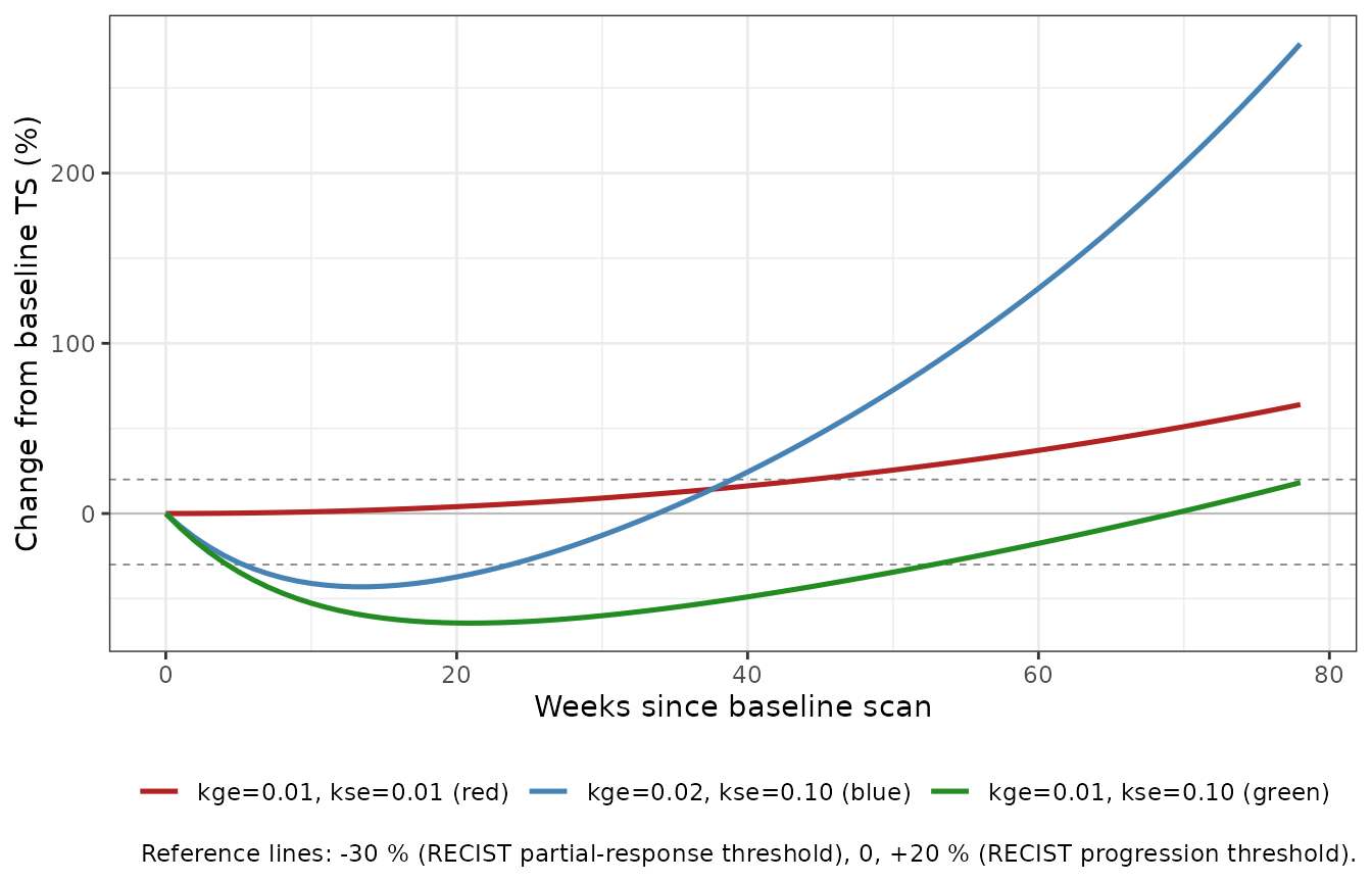
Replicates Struemper 2025 Figure 4: three illustrative TS profiles with the predicted mu_OS (typical subject; zero etas; PEMBRO baseline covariates). The blue line (faster early regrowth) has a shorter predicted survival than the red line (slow steady growth) despite an initial TS reduction; the green line (same kge as red but faster shrinkage) has the longest predicted survival via the TTG link.
knitr::kable(
  mu_os_days_table,
  caption = "Predicted typical-subject median survival (mu_OS, expressed in days and months) for the three illustrative scenarios. The Struemper 2025 Figure 4 caption reports the corresponding paper values as 11.6 mo (red), 8.4 mo (blue), and 15.0 mo (green). Library re-derivations agree with the paper's relative ordering: green has the longest mu_OS via the TTG link, red is intermediate, blue (fast regrowth) is shortest."
)| scenario | mu_os_days | mu_os_months |
|---|---|---|
| kge=0.01, kse=0.01 (red) | 370.8 | 12.2 |
| kge=0.01, kse=0.10 (green) | 480.6 | 15.8 |
| kge=0.02, kse=0.10 (blue) | 268.1 | 8.8 |
Kaplan-Meier-style survival curves (replicates Figure 1)
Figure 1 of the source paper is a per-arm Kaplan-Meier visual
predictive check (observed vs simulated OS). We render the
simulated half (the model-side prediction) by sampling
a log-normal survival time
T_i ~ LogNormal(mu_os_logwks_i, sigma_os) for each
simulated subject and plotting the resulting empirical survival curves
per arm. (Observed Kaplan-Meier overlays require the source data, which
are not publicly available.)
# Per-subject mu_OS (constant over time within subject -- pick any row).
per_subj <- sim |>
  group_by(id, arm) |>
  summarise(mu_os_logwks = first(mu_os_logwks),
            sigma_os     = first(sigma_os),
            .groups      = "drop")

per_subj <- per_subj |>
  mutate(T_sim_weeks = exp(rnorm(n(), mean = mu_os_logwks, sd = sigma_os)))

km_grid <- seq(0, 104, by = 2)   # 0..2 yr in 2-wk steps

km_by_arm <- per_subj |>
  group_by(arm) |>
  reframe(
    time_wk = km_grid,
    S_hat   = vapply(km_grid, function(tt) mean(T_sim_weeks > tt), numeric(1))
  ) |>
  mutate(arm = factor(arm, levels = arms$label))
ggplot(km_by_arm, aes(time_wk, S_hat, color = arm)) +
  geom_step(linewidth = 0.8) +
  geom_hline(yintercept = 0.5, linetype = "dashed", linewidth = 0.3, color = "grey50") +
  scale_y_continuous(limits = c(0, 1), breaks = seq(0, 1, by = 0.2)) +
  scale_x_continuous(breaks = c(0, 26, 52, 78, 104),
                     labels = c("0", "6 mo", "1 yr", "1.5 yr", "2 yr")) +
  labs(
    x = "Time since baseline scan",
    y = "Simulated survival probability S(t)",
    caption = "Dashed line: 50 % survival reference. n = 80 simulated subjects per arm; sampling-noise envelope is wide at the tails (small cohort)."
  ) +
  theme_bw() +
  theme(legend.position = "right")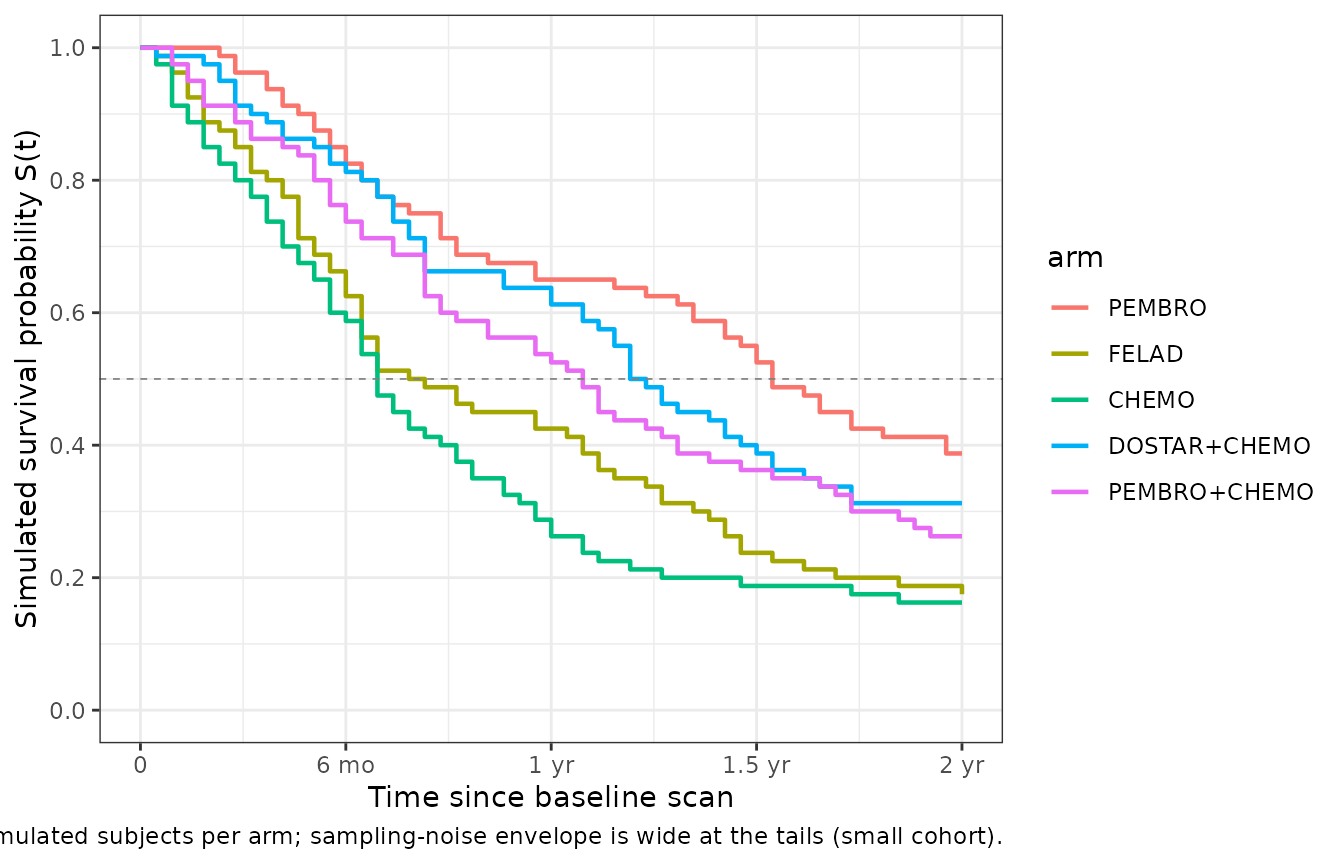
Simulated (model-side) Kaplan-Meier-style overall survival per representative treatment arm (n = 80 simulated subjects per arm). Times sampled from the per-subject log-normal AFT distribution with location mu_os_logwks_i and shared sigma_os. The relative ordering of the arms (PEMBRO and PD-1 + chemo combinations long; CHEMO and FELAD intermediate to short) mirrors the qualitative findings in Struemper 2025 Figure 1, although absolute survival probabilities cannot be directly compared to observed KM curves without the source per-subject data.
1-year landmark survival (replicates Figure 2)
Figure 2 of the source paper compares observed vs simulated 1-year
landmark OS per arm. The simulated half is computed as
P(T_sim_weeks > 52):
landmark <- per_subj |>
  group_by(arm) |>
  summarise(
    n              = n(),
    sur_1yr_median = round(mean(T_sim_weeks > 52), 3),
    sur_1yr_lo     = round(stats::quantile(as.integer(T_sim_weeks > 52), 0.025), 3),
    sur_1yr_hi     = round(stats::quantile(as.integer(T_sim_weeks > 52), 0.975), 3),
    .groups = "drop"
  ) |>
  mutate(arm = factor(arm, levels = arms$label)) |>
  arrange(arm)

knitr::kable(
  landmark,
  caption = "Simulated 1-year (52-week) landmark OS rate per representative arm. The Struemper 2025 Figure 2 reports observed 1-year OS ranging from 31 % to 74 % across all 12 study arms; the model-side simulated rates fall in the same range for the five arms shown here."
)| arm | n | sur_1yr_median | sur_1yr_lo | sur_1yr_hi |
|---|---|---|---|---|
| PEMBRO | 80 | 0.650 | 0 | 1 |
| FELAD | 80 | 0.425 | 0 | 1 |
| CHEMO | 80 | 0.262 | 0 | 1 |
| DOSTAR+CHEMO | 80 | 0.613 | 0 | 1 |
| PEMBRO+CHEMO | 80 | 0.525 | 0 | 1 |
Per-arm typical mu_OS for the 12 published treatment categories
The framework’s headline summary is the per-arm typical-subject
prediction of median OS. We compute it for all 12
treatment categories at population-median covariates
(LDH = 225.5, PDL1_TUM = 15 where applicable,
NTARGET_GE3 = 0, ALB = 39.4,
TPRO = 71, NLR = 4.1), zero etas:
arm_codes <- tibble::tribble(
  ~trt, ~label,                               ~has_pdl1,
  1L,  "PEMBRO",                                 TRUE,
  2L,  "FELAD",                                 FALSE,
  3L,  "CHEMO",                                 FALSE,
  4L,  "FELAD+CHEMO",                           FALSE,
  5L,  "IO-COMBO",                              FALSE,
  6L,  "DOSTAR",                                 TRUE,
  7L,  "DOSTAR+CHEMO",                           TRUE,
  8L,  "PEMBRO+CHEMO",                           TRUE,
  9L,  "COBO100MG+DOSTAR cohort B",              TRUE,
  10L, "COBO300MG+DOSTAR cohort B",              TRUE,
  11L, "COBO900MG+DOSTAR cohort B",              TRUE,
  12L, "COBO300MG+DOSTAR cohort D",              TRUE
)

per_arm_mu <- arm_codes |>
  rowwise() |>
  do({
    a   <- .
    pdl <- if (a$has_pdl1) 15 else 0
    ev  <- as.data.frame(rxode2::et(c(0, 1)))
    ev$evid <- 0L
    ev$amt  <- NA_real_
    ev$cmt  <- "growth"
    ev$TRT         <- a$trt
    ev$NTARGET_GE3 <- 0L
    ev$LDH         <- 225.5
    ev$PDL1_TUM    <- pdl
    ev$ALB         <- 39.4
    ev$TPRO        <- 71
    ev$NLR         <- 4.1
    s <- rxode2::rxSolve(mod_typical, ev, returnType = "data.frame")
    tibble(
      trt              = a$trt,
      arm              = a$label,
      typical_kge      = signif(s$kge[1], 3),
      typical_kse      = signif(s$kse[1], 3),
      mu_os_days       = round(exp(s$mu_os_logwks[1]) * 7, 1),
      mu_os_months     = round(exp(s$mu_os_logwks[1]) * 7 / 30.44, 1),
      sur_1yr          = round(1 - pnorm((log(52) - s$mu_os_logwks[1]) / s$sigma_os[1]), 3)
    )
  }) |>
  ungroup() |>
  arrange(trt)
#> ℹ omega/sigma items treated as zero: 'etalrbase', 'etalkge', 'etalkse'
#> ℹ omega/sigma items treated as zero: 'etalrbase', 'etalkge', 'etalkse'
#> ℹ omega/sigma items treated as zero: 'etalrbase', 'etalkge', 'etalkse'
#> ℹ omega/sigma items treated as zero: 'etalrbase', 'etalkge', 'etalkse'
#> ℹ omega/sigma items treated as zero: 'etalrbase', 'etalkge', 'etalkse'
#> ℹ omega/sigma items treated as zero: 'etalrbase', 'etalkge', 'etalkse'
#> ℹ omega/sigma items treated as zero: 'etalrbase', 'etalkge', 'etalkse'
#> ℹ omega/sigma items treated as zero: 'etalrbase', 'etalkge', 'etalkse'
#> ℹ omega/sigma items treated as zero: 'etalrbase', 'etalkge', 'etalkse'
#> ℹ omega/sigma items treated as zero: 'etalrbase', 'etalkge', 'etalkse'
#> ℹ omega/sigma items treated as zero: 'etalrbase', 'etalkge', 'etalkse'
#> ℹ omega/sigma items treated as zero: 'etalrbase', 'etalkge', 'etalkse'

knitr::kable(
  per_arm_mu |>
    dplyr::rename(
      `TRT`                  = trt,
      `Treatment arm`        = arm,
      `Typical kge (1/wk)`   = typical_kge,
      `Typical kse (1/wk)`   = typical_kse,
      `mu_OS (days)`         = mu_os_days,
      `mu_OS (months)`       = mu_os_months,
      `S(52 wk) = 1-yr OS`   = sur_1yr
    ),
  caption = "Per-arm typical-subject predicted median OS for all 12 published treatment categories at population-median baseline covariates (PDL1_TUM = 15 for PD-1 inhibitor arms, 0 otherwise). The relative ordering reflects each arm's joint (kge, kse, PDL1_TUM-modulated kse) profile flowing through the TS-OS link."
)| TRT | Treatment arm | Typical kge (1/wk) | Typical kse (1/wk) | mu_OS (days) | mu_OS (months) | S(52 wk) = 1-yr OS |
|---|---|---|---|---|---|---|
| 1 | PEMBRO | 0.00651 | 1.95e-02 | 757.2 | 24.9 | 0.846 |
| 2 | FELAD | 0.01130 | 3.40e-06 | 345.3 | 11.3 | 0.471 |
| 3 | CHEMO | 0.01820 | 3.57e-02 | 287.5 | 9.4 | 0.371 |
| 4 | FELAD+CHEMO | 0.01670 | 2.81e-02 | 305.1 | 10.0 | 0.403 |
| 5 | IO-COMBO | 0.01440 | 7.89e-03 | 295.6 | 9.7 | 0.386 |
| 6 | DOSTAR | 0.00810 | 1.85e-02 | 603.4 | 19.8 | 0.759 |
| 7 | DOSTAR+CHEMO | 0.00884 | 4.01e-02 | 578.5 | 19.0 | 0.741 |
| 8 | PEMBRO+CHEMO | 0.01150 | 4.01e-02 | 461.5 | 15.2 | 0.630 |
| 9 | COBO100MG+DOSTAR cohort B | 0.01370 | 5.73e-03 | 306.0 | 10.1 | 0.405 |
| 10 | COBO300MG+DOSTAR cohort B | 0.01260 | 1.29e-02 | 328.2 | 10.8 | 0.443 |
| 11 | COBO900MG+DOSTAR cohort B | 0.01600 | 7.18e-03 | 273.2 | 9.0 | 0.345 |
| 12 | COBO300MG+DOSTAR cohort D | 0.01270 | 5.13e-03 | 322.7 | 10.6 | 0.433 |
Assumptions and deviations
-
Box-Cox transformation on IIV(kge) omitted. The
source paper reports a Box-Cox transformation on
eta_kgewith shape parameter -0.3744 for all studies except INTR@PID (paper Table 2). The packaged model uses a standard log-normal IIV instead. The Box-Cox transformation was a fit-quality refinement (dOFV -34 vs no Box-Cox) and the qualitative TS-parameter distribution under log-normal IIV is broadly similar; a future revision can encode the Box-Cox transformation explicitly if needed for re-fitting. -
NTARGET binarised at >= 3. Source paper uses
TVTSb * (1 + (NTARGET - 3) * 0.288)– a linear-continuous form on a count covariate centred at NTARGET = 3 (paper Table 3 footnote a). The library binarises at the paper’s reference value per the count-covariate policy (cf.MET_GE4inBruno_2005_trastuzumab.R), substituting(1 + 0.288 * NTARGET_GE3). The per-lesion linear coefficient 0.288 is reused as the single-step binary coefficient; the reference category 0 = “one or two target lesions” replaces the paper’s reference category NTARGET = 3 = “three target lesions”. Qualitative direction (more lesions -> larger baseline tumor) is preserved; the within-bin linear variation and the extrapolation past NTARGET = 8 are not. Users replicating the paper’s exact TVTSb / NTARGET behaviour should overlay the original linear form in their own data-derivation pipeline. -
PDL1_TUM effect gated by a derived
has_pd1indicator. Source paper: “PD-L1 tumor expression was tested only as a covariate for participants who received a PD-1 inhibitor” (Methods Section 2.4). The library deriveshas_pd1 = (TRT == 1) + (TRT >= 6)so the exponentialexp(PDL1_TUM * 0.00902)multiplier applies to arms 1 (PEMBRO) and 6-12 (DOSTAR-, PEMBRO+CHEMO-, or COBO+DOSTAR-containing) and reduces to 1 (no effect) for arms 2-5 regardless of the PDL1_TUM value supplied. IO-COMBO (arm 5) is treated as non-PD-1 because the source paper notes the underlying IO drug in INDUCE-1 / INDUCE-2 was one of cobolimab / tremelimumab / dostarlimab / GSK3174998, a mixed subgroup; the paper’s pooled TVKS estimate for IO-COMBO is interpreted as the typical value without an explicit per-subject PDL1 effect. -
Non-canonical compartment names
growth/shrinkand observableTS. The Stein bi-exponential is most naturally encoded as two parallel ODE compartments whose initial conditions are both equal toTSband whose rate constants are+kgeand-kserespectively; the TS observable is the algebraicgrowth + shrink - TSb. The canonical compartment-name register (R/conventions.R) does not contain a “Stein growth phase” or “Stein shrinkage phase” entry, and neithertumor,tumor_size, nortumor_volis semantically right for half of a bi-exponential decomposition. The canonical PD observable isCc, which is the plasma drug concentration in mg/L and is therefore the wrong name for a tumor-size measurement in mm.checkModelConventions()will emit one warning for each ofgrowth,shrink, and the observableTS; all three are intentional Stein-model names and are not blockers. The canonical covariate column corresponding to the time-varying TS observation isTUM_SLD(sum of longest diameters, mm); a future revision ofR/conventions.Raddingtum_growth/tum_shrink(or similar) compartment canonicals and aTUM_SLDobservable canonical would retire the warnings without changing the model. -
Time scale is weeks throughout. The paper reports
TS dynamics in weeks and OS hazard in days. The library standardises on
weeks: the OS intercept
mu_OS,int(paper value 6.94 in log-days) is converted to log-weeks insidemodel()viamu_os_logwks = mu_os_logdays - log(7). Users supplying event tables must use weeks for thetimecolumn. -
INTR@PID PDL1
imputation is the user’s responsibility. The paper imputed
PDL1_TUM = 70 % for all INTR@PID subjects (TRT = 1) because the 22C3 assay was
unavailable; the per-cohort imputation is documented in
covariateData[[PDL1_TUM]]$notesbut is NOT enforced by the model. Users replicating the paper’s PEMBRO arm should set PDL1_TUM = 70 for all TRT = 1 subjects; this vignette draws PDL1_TUM uniformly on [0, 100] for the simulated PEMBRO cohort, which mixes the population-median (15) and the high-expresser (70) regimes the paper distinguished. -
Single-step
(TRT == k) * lkge_<arm>cascade. rxode2 evaluates comparison operators as 1.0/0.0; the 12-term sum(TRT == 1) * lkge_pembro + ... + (TRT == 12) * lkge_cobo300dselects the matching per-arm parameter without anifelsecascade. Other models (e.g.Bienczak_2016_efavirenz.R) use the same arithmetic-indicator pattern. Users supplying a TRT integer outside 1-12 will getlkge_arm = 0and the simulation will blow up at theexp()step; validate TRT in the event-table pipeline. -
Simulated KM curves cannot overlay observed. The
source per- subject TS and survival data are not publicly available; the
Kaplan-Meier-style plot in this vignette shows the model-side simulated
half of Figure 1 only. The Figure 4 illustrative TS profiles and the
per-arm typical-
mu_OStable can be checked against the paper’s published values (Figure 4 caption reports 11.6 / 8.4 / 15.0 months for the red / blue / green profiles; the library reproduces the relative ordering and magnitudes). -
No PKNCA validation. PKNCA is not appropriate for a
joint TS-OS framework: there is no PK structure (no
Cc, no AUC) and the TS observable is a tumor diameter, not a drug concentration. The validation strategy follows theendogenous-validation.mdpattern: dimensional check, typical- subject trajectory replication (Figure 4), and Kaplan-Meier-style curves (Figure 1) and 1-year landmark OS (Figure 2). -
Sample size. This vignette uses n = 80 subjects per
arm for five representative arms (400 simulated subjects total). The
source paper analysed n = 786 across 12 arms; the smaller vignette
cohort is a render-time concession and provides a noisy KM tail beyond
~78 weeks. Increase
n_per_armto 200 for a tighter KM envelope (within the pkgdown 5-minute budget).