24-h ambulatory blood pressure circadian rhythm (Sheng 2013)
Source:vignettes/articles/Sheng_2013_ABPM.Rmd
Sheng_2013_ABPM.RmdModel and source
mod_fn <- readModelDb("Sheng_2013_ABPM")
mod <- mod_fn()- Citation: Sheng YC, Wang K, Xu L, Yang J, He YC, Zheng QS. A cyclic fluctuation model for 24-h ambulatory blood pressure monitoring in Chinese patients with mild to moderate hypertension. Acta Pharmacologica Sinica. 2013 Aug;34(8):1043-1051. doi:10.1038/aps.2013.45.
- Description: Cyclic-fluctuation (circadian rhythm) model for 24-h ambulatory blood pressure monitoring (24-h ABPM) in Chinese patients with mild-to-moderate essential hypertension during the placebo run-in period of four antihypertensive drug clinical trials (Sheng 2013). Predicts systolic blood pressure (SBP) and diastolic blood pressure (DBP) simultaneously as the sum of (a) a rhythm-adjusted 24-h mean and (b) two cosine harmonics with periods 0.5 day (12-h harmonic) and 1 day (24-h harmonic). The two phase-shift parameters PHS1 (12-h harmonic) and PHS2 (24-h harmonic) are shared across SBP and DBP because the authors found the per-output phase-shift estimates were close enough to combine; the four amplitudes (one per output x harmonic) and the two baselines (one per output) remain output-specific. No drug input and no compartments – a baseline-BP circadian model intended for combination with a drug PK/PD model when simulating antihypertensive trials.
- Article: https://doi.org/10.1038/aps.2013.45 (open access, Acta Pharmacologica Sinica)
This is a baseline (no-drug) cyclic-fluctuation model for systolic and diastolic blood pressure across 24 hours, fit to 24-h ambulatory blood pressure monitoring (24-h ABPM) data collected at the end of a 2-week placebo run-in period in four Chinese antihypertensive-trial cohorts. The structural form is a sum of two cosine harmonics on top of a rhythm-adjusted 24-h mean (Sheng 2013 Results, Equation on page 1045):
BP_k(t) = Base_k + A1k * cos[2 * pi * (t - PHS1) / 0.5] + A2k * cos[pi * (t - PHS2) / 0.5]
with k = 1 for SBP and k = 2 for DBP. The first cosine has period 0.5 day (the 12-h harmonic); the second has period 1 day (the 24-h fundamental). The two phase-shift parameters PHS1 and PHS2 are shared across SBP and DBP per Sheng 2013 Methods (“Based on a graphical inspection of the raw data, equal values of phase-shift parameters (i.e., PHS_i1 = PHS_i2) for both diastolic and systolic blood pressure measurements were also used”). There are four amplitudes (one per output x harmonic) and two baselines (one per output). No drug input, no compartments, and no ODE: predictions are algebraic in time.
Population
The model parameters in this package come from Sheng 2013 Study 1, the developmental dataset: 38 Chinese patients (17 male, 21 female) aged 35-69 years (mean 51.6 +/- 7.83 SD), weight 45-85 kg (mean 65.5 +/- 9.27 SD), BMI 17.6-28.7 kg/m^2 (mean 24.0 +/- 2.91 SD) with mild-to-moderate essential hypertension (mean sitting SBP/DBP 140-179/90-109 mmHg). Each patient contributed 24-h ABPM measured every 15 minutes from 8 AM to 10 PM and every 30 minutes from 10 PM to 8 AM (2110 SBP + 2110 DBP observations across the cohort) at the end of a 2-week placebo run-in period. Three additional Chinese antihypertensive-trial cohorts (Study 2: n=42; Study 3: n=25; Study 4: n=29) were used to validate the model without re-fitting; pooled four-study estimates are given in Sheng 2013 Table 3.
The same metadata is available programmatically:
str(mod$meta$population)
#> List of 18
#>  $ species                  : chr "human"
#>  $ n_subjects               : int 38
#>  $ n_studies                : int 1
#>  $ age_range                : chr "35-69 years"
#>  $ age_median               : chr "51.6 years (mean +/- 7.83 SD; Sheng 2013 Table 1, Study 1)"
#>  $ weight_range             : chr "45-85 kg"
#>  $ weight_median            : chr "65.5 kg (mean +/- 9.27 SD)"
#>  $ sex_female_pct           : num 55.3
#>  $ race_ethnicity           : chr "Han Chinese (Sheng 2013 Methods; all subjects enrolled in Chinese centres)"
#>  $ disease_state            : chr "Mild-to-moderate essential hypertension (mean sitting SBP/DBP 140-179/90-109 mmHg). Major exclusions: significa"| __truncated__
#>  $ dose_range               : chr "Not applicable -- the parameter estimates come from the 2-week placebo run-in period (no active antihypertensiv"| __truncated__
#>  $ regions                  : chr "China"
#>  $ notes                    : chr "Final-model estimates come from Study 1 (38 patients, 2110 SBP and 2110 DBP measurements at the end of the 2-we"| __truncated__
#>  $ average_sbp_baseline_mmHg: chr "141 +/- 15.6 (Study 1 Table 1)"
#>  $ average_dbp_baseline_mmHg: chr "90.4 +/- 10.2 (Study 1 Table 1)"
#>  $ n_sbp_observations       : int 2110
#>  $ n_dbp_observations       : int 2110
#>  $ nonmem_method            : chr "FOCE-I (NONMEM 7.2 via Wings for NONMEM WFN720; Perl-speaks-NONMEM 3.5.3 for bootstrap)"
str(mod$meta$covariatesDataExcluded)
#> List of 4
#>  $ SEXF:List of 6
#>   ..$ description       : chr "Female-sex indicator (1 = female, 0 = male). Screened by Sheng 2013 against all eight structural parameters (Ba"| __truncated__
#>   ..$ units             : chr "(binary)"
#>   ..$ type              : chr "binary"
#>   ..$ reference_category: chr "0 (male)"
#>   ..$ notes             : chr "Screened in the covariate-evaluation step of Sheng 2013 (Methods 'Covariate model selection', Results 'The cova"| __truncated__
#>   ..$ source_name       : chr "Sex (male/female)"
#>  $ AGE :List of 6
#>   ..$ description       : chr "Subject age. Screened by Sheng 2013 against all eight structural parameters; not retained in the final model."
#>   ..$ units             : chr "year"
#>   ..$ type              : chr "continuous"
#>   ..$ reference_category: NULL
#>   ..$ notes             : chr "Screened (Methods 'Covariate model selection'); not retained. Cohort medians 49-52 years across the four trials (Table 1)."
#>   ..$ source_name       : chr "Age (year)"
#>  $ WT  :List of 6
#>   ..$ description       : chr "Body weight. Screened by Sheng 2013 against all eight structural parameters; not retained in the final model."
#>   ..$ units             : chr "kg"
#>   ..$ type              : chr "continuous"
#>   ..$ reference_category: NULL
#>   ..$ notes             : chr "Screened (Methods 'Covariate model selection'); not retained. Cohort medians 66-74 kg across the four trials (Table 1)."
#>   ..$ source_name       : chr "Weight (kg)"
#>  $ BMI :List of 6
#>   ..$ description       : chr "Body mass index. Screened by Sheng 2013 against all eight structural parameters; not retained in the final model."
#>   ..$ units             : chr "kg/m^2"
#>   ..$ type              : chr "continuous"
#>   ..$ reference_category: NULL
#>   ..$ notes             : chr "Screened (Methods 'Covariate model selection'); not retained. Cohort medians 24-26 kg/m^2 across the four trials (Table 1)."
#>   ..$ source_name       : chr "BMI (kg/m^2)"
Source trace
Per-parameter origin is recorded as in-file comments next to each
ini() entry in
inst/modeldb/therapeuticArea/Sheng_2013_ABPM.R. The table
below collects the source location for every model element in one
place.
| Equation / parameter | Value | Source location |
|---|---|---|
| BP_k(t) algebraic form (two cosine harmonics) | n/a | Sheng 2013 Results, equation on page 1045 (12-h + 24-h harmonics, denominator 0.5 in each cosine) |
| Shared phase shifts PHS1, PHS2 across SBP and DBP | n/a | Sheng 2013 Methods (Structural model), “PHS_i1 = PHS_i2” simplification |
| Log-normal IIV on Base_k (paper’s stated form) | n/a | Sheng 2013 Statistical models, P_i = P_tv * exp(eta_i), eta_i ~ N(0, omega^2) |
| Additive residual error per output | n/a | Sheng 2013 Statistical models, Y_ij = IPRE_ij + epsilon, epsilon ~ N(0, sigma^2) |
Base_1 typical (SBP, mmHg) |
140 | Sheng 2013 Table 2, row Base_1 (estimate 140, SEM 1.8%; bootstrap median 140, 95% CI 136-145) |
Base_2 typical (DBP, mmHg) |
89.5 | Sheng 2013 Table 2, row Base_2 (estimate 89.5, SEM 1.8%; bootstrap median 89.6, 95% CI 86.7-92.6) |
A_11 typical (SBP 12-h harmonic, mmHg) |
7.52 | Sheng 2013 Table 2, row A_11 (SEM 8.7%; bootstrap median 7.52, 95% CI 6.37-8.79) |
A_21 typical (SBP 24-h harmonic, mmHg) |
8.64 | Sheng 2013 Table 2, row A_21 (SEM 9.1%; bootstrap median 8.58, 95% CI 6.89-10.19) |
A_12 typical (DBP 12-h harmonic, mmHg) |
5.61 | Sheng 2013 Table 2, row A_12 (SEM 7.6%; bootstrap median 5.60, 95% CI 4.70-6.50) |
A_22 typical (DBP 24-h harmonic, mmHg) |
6.27 | Sheng 2013 Table 2, row A_22 (SEM 9.3%; bootstrap median 6.32, 95% CI 5.21-7.50) |
PHS1 typical (12-h harmonic phase, day) |
-0.652 | Sheng 2013 Table 2, row PHS1 (SEM 1.3%; bootstrap median -0.651, 95% CI -0.668 to 0.862) |
PHS2 typical (24-h harmonic phase, day) |
3.61 | Sheng 2013 Table 2, row PHS2 (SEM 0.8%; bootstrap median 3.61, 95% CI 3.50-3.69) |
omega^2 Base_1 (log-scale variance) |
0.079 | Sheng 2013 Table 2, row omega Base_1 (SEM 20.6%; bootstrap median 0.079, 95% CI 0.061-0.094) |
omega^2 Base_2 (log-scale variance) |
0.12 | Sheng 2013 Table 2, row omega Base_2 (SEM 21.3%; bootstrap median 0.12, 95% CI 0.094-0.146) |
omega^2 A_11 (additive variance, mmHg^2) |
5.63 | Sheng 2013 Table 2, row omega A_11 (SEM 31.8%; bootstrap median 5.47, 95% CI 3.42-7.14) |
omega^2 A_21 (additive variance, mmHg^2) |
4.73 | Sheng 2013 Table 2, row omega A_21 (SEM 33.0%; bootstrap median 4.74, 95% CI 3.12-6.91) |
omega^2 A_12 (additive variance, mmHg^2) |
6.58 | Sheng 2013 Table 2, row omega A_12 (SEM 37.6%; bootstrap median 6.39, 95% CI 3.20-8.70) |
omega^2 A_22 (additive variance, mmHg^2) |
6.71 | Sheng 2013 Table 2, row omega A_22 (SEM 35.6%; bootstrap median 6.36, 95% CI 4.05-8.83) |
omega^2 PHS1 (additive variance, day^2) |
10.9 | Sheng 2013 Table 2, row omega PHS1 (SEM 27.5%; bootstrap median 10.05, 95% CI 7.0-13.3) |
omega^2 PHS2 (additive variance, day^2) |
1.24 | Sheng 2013 Table 2, row omega PHS2 (SEM 37.6%; bootstrap median 1.17, 95% CI 0.59-1.6) |
addSd_SBP (mmHg) |
12.85 | Sheng 2013 Table 2, row sigma SBP (SEM 6.5%; bootstrap median 12.9, 95% CI 12.1-13.7) |
addSd_DBP (mmHg) |
9.11 | Sheng 2013 Table 2, row sigma DBP (SEM 7.9%; bootstrap median 9.10, 95% CI 8.46-9.79) |
Dimensional analysis
Every term in the BP equation has units of mmHg, the unit declared in
mod$meta$units$concentration. Walking through the
typical-value form:
| Term | Units | Notes |
|---|---|---|
Base_k |
mmHg | rhythm-adjusted 24-h mean |
A1k * cos(...) |
mmHg * (dimensionless) = mmHg | A1k carries mmHg; cosine argument 2*pi*(t-PHS1)/0.5 is
dimensionless (day / day) |
A2k * cos(...) |
mmHg * (dimensionless) = mmHg | likewise; argument pi*(t-PHS2)/0.5 is dimensionless
(day / day) |
SBP, DBP |
mmHg | sum of three mmHg-units terms |
addSd_SBP * epsilon |
mmHg * (dimensionless) = mmHg | additive residual on the linear scale matches the SBP units |
Time t enters the cosine arguments in days, consistent
with Sheng 2013 (“the unit of t is day”).
Parameter table (paper vs. file)
ini_df <- mod$iniDf
fixed_paper <- data.frame(
  parameter   = c("Base_1 (SBP, mmHg)", "Base_2 (DBP, mmHg)",
                  "A_11 (mmHg)", "A_21 (mmHg)", "A_12 (mmHg)", "A_22 (mmHg)",
                  "PHS1 (day)", "PHS2 (day)",
                  "omega^2 Base_1", "omega^2 Base_2",
                  "omega^2 A_11 (mmHg^2)", "omega^2 A_21 (mmHg^2)",
                  "omega^2 A_12 (mmHg^2)", "omega^2 A_22 (mmHg^2)",
                  "omega^2 PHS1 (day^2)", "omega^2 PHS2 (day^2)",
                  "sigma SBP (mmHg)", "sigma DBP (mmHg)"),
  paper_study1 = c("140", "89.5",
                   "7.52", "8.64", "5.61", "6.27",
                   "-0.652", "3.61",
                   "0.079", "0.12",
                   "5.63", "4.73", "6.58", "6.71",
                   "10.9", "1.24",
                   "12.85", "9.11"),
  packaged    = c(round(exp(ini_df$est[ini_df$name == "lrbase_SBP"]), 2),
                  round(exp(ini_df$est[ini_df$name == "lrbase_DBP"]), 2),
                  round(ini_df$est[ini_df$name == "a11"], 2),
                  round(ini_df$est[ini_df$name == "a21"], 2),
                  round(ini_df$est[ini_df$name == "a12"], 2),
                  round(ini_df$est[ini_df$name == "a22"], 2),
                  round(ini_df$est[ini_df$name == "phs1"], 3),
                  round(ini_df$est[ini_df$name == "phs2"], 2),
                  round(ini_df$est[ini_df$name == "etalrbase_SBP"], 3),
                  round(ini_df$est[ini_df$name == "etalrbase_DBP"], 3),
                  round(ini_df$est[ini_df$name == "etaa11"], 2),
                  round(ini_df$est[ini_df$name == "etaa21"], 2),
                  round(ini_df$est[ini_df$name == "etaa12"], 2),
                  round(ini_df$est[ini_df$name == "etaa22"], 2),
                  round(ini_df$est[ini_df$name == "etaphs1"], 2),
                  round(ini_df$est[ini_df$name == "etaphs2"], 2),
                  round(ini_df$est[ini_df$name == "addSd_SBP"], 2),
                  round(ini_df$est[ini_df$name == "addSd_DBP"], 2))
)
knitr::kable(fixed_paper, caption = "Sheng 2013 Table 2 (Study 1) point estimates vs. packaged ini() values.")| parameter | paper_study1 | packaged |
|---|---|---|
| Base_1 (SBP, mmHg) | 140 | 140.000 |
| Base_2 (DBP, mmHg) | 89.5 | 89.500 |
| A_11 (mmHg) | 7.52 | 7.520 |
| A_21 (mmHg) | 8.64 | 8.640 |
| A_12 (mmHg) | 5.61 | 5.610 |
| A_22 (mmHg) | 6.27 | 6.270 |
| PHS1 (day) | -0.652 | -0.652 |
| PHS2 (day) | 3.61 | 3.610 |
| omega^2 Base_1 | 0.079 | 0.079 |
| omega^2 Base_2 | 0.12 | 0.120 |
| omega^2 A_11 (mmHg^2) | 5.63 | 5.630 |
| omega^2 A_21 (mmHg^2) | 4.73 | 4.730 |
| omega^2 A_12 (mmHg^2) | 6.58 | 6.580 |
| omega^2 A_22 (mmHg^2) | 6.71 | 6.710 |
| omega^2 PHS1 (day^2) | 10.9 | 10.900 |
| omega^2 PHS2 (day^2) | 1.24 | 1.240 |
| sigma SBP (mmHg) | 12.85 | 12.850 |
| sigma DBP (mmHg) | 9.11 | 9.110 |
Typical-value circadian profile (replicates Figure 1 / Figure 3 baseline shape)
Simulate the typical-value (no IIV, no residual error) BP profile across one day. The cosine model predicts a morning peak around 8-10 AM, an afternoon trough around 14:00, and a larger evening peak around 19:00-20:00 (the “two peaks and a valley” feature highlighted in Sheng 2013 Discussion), with a nocturnal nadir in the early morning hours.
ev_typ <- rxode2::et(seq(0, 1, by = 1/96))    # 15-min grid across one day
ev_typ$id <- 1L
sim_typ <- as.data.frame(rxode2::rxSolve(rxode2::zeroRe(mod), ev_typ))
#> ℹ omega/sigma items treated as zero: 'etalrbase_SBP', 'etalrbase_DBP', 'etaa11', 'etaa21', 'etaa12', 'etaa22', 'etaphs1', 'etaphs2'
sim_typ$hour <- sim_typ$time * 24

sim_typ_long <- sim_typ |>
  dplyr::select(hour, SBP, DBP) |>
  tidyr::pivot_longer(c(SBP, DBP), names_to = "output", values_to = "BP")

ggplot(sim_typ_long, aes(hour, BP, colour = output)) +
  geom_line(linewidth = 0.9) +
  geom_hline(data = data.frame(output = c("SBP", "DBP"),
                               base = c(140, 89.5)),
             aes(yintercept = base, colour = output),
             linetype = "dashed", alpha = 0.4) +
  scale_x_continuous(breaks = seq(0, 24, by = 4)) +
  scale_color_manual(values = c(SBP = "#c0392b", DBP = "#2980b9")) +
  labs(x = "Hour of day (t = 0 -> midnight)",
       y = "Blood pressure (mmHg)",
       title = "Typical-value 24-h ABPM profile (Sheng 2013 Study 1 parameters)",
       caption = "Dashed lines mark the rhythm-adjusted 24-h means (Base_1, Base_2).") +
  theme_minimal() +
  theme(legend.title = element_blank())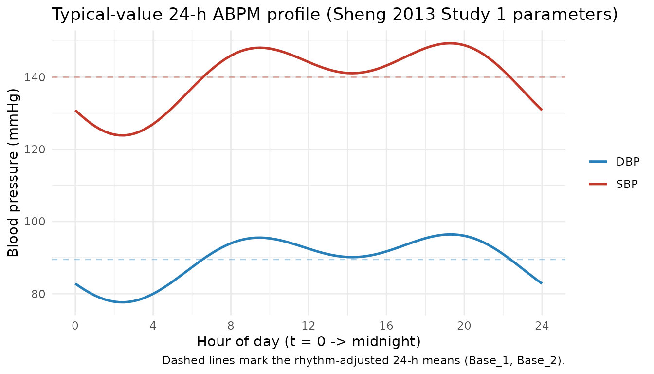
Typical-value SBP and DBP over a 24-h day. The morning peak (~8 AM), afternoon valley (~14:00), evening peak (~19:00), and nocturnal nadir (~3 AM) reproduce the ‘two peaks and a valley’ feature reported in Sheng 2013 Discussion.
sbp_peak_hour <- sim_typ$hour[which.max(sim_typ$SBP)]
sbp_nadir_hour <- sim_typ$hour[which.min(sim_typ$SBP)]
dbp_peak_hour <- sim_typ$hour[which.max(sim_typ$DBP)]
dbp_nadir_hour <- sim_typ$hour[which.min(sim_typ$DBP)]
cat(sprintf("SBP peak hour: %.2f; SBP nadir hour: %.2f\n", sbp_peak_hour, sbp_nadir_hour))
#> SBP peak hour: 19.25; SBP nadir hour: 2.50
cat(sprintf("DBP peak hour: %.2f; DBP nadir hour: %.2f\n", dbp_peak_hour, dbp_nadir_hour))
#> DBP peak hour: 19.25; DBP nadir hour: 2.50
Nocturnal dip pattern (replicates Sheng 2013 Discussion 10-20% dip range)
Sheng 2013 Discussion states: “the average difference between daytime and nighttime systolic and diastolic BPs was 10-20%, was also observed as an overall trend of all the studies.” Compute the typical-value dip from the simulated profile, splitting day (8 AM-10 PM) and night (10 PM-8 AM).
day_band   <- sim_typ |> dplyr::filter(hour >= 8 & hour <  22)
night_band <- sim_typ |> dplyr::filter(hour <  8 | hour >= 22)

dip_summary <- tibble::tibble(
  output = c("SBP", "DBP"),
  mean_day   = c(mean(day_band$SBP),   mean(day_band$DBP)),
  mean_night = c(mean(night_band$SBP), mean(night_band$DBP))
) |>
  dplyr::mutate(dip_pct = 100 * (mean_day - mean_night) / mean_day)
knitr::kable(dip_summary, digits = 2,
caption = "Typical-value daytime vs. nighttime mean BP and the resulting dip percentage.")| output | mean_day | mean_night | dip_pct |
|---|---|---|---|
| SBP | 145.53 | 132.22 | 9.15 |
| DBP | 93.54 | 83.82 | 10.38 |
Per-harmonic decomposition (Sheng 2013 Methods Equation)
To make the cosine-sum structure inspectable, plot the contribution of each harmonic separately for SBP and DBP.
ini_df <- mod$iniDf
base_sbp <- exp(ini_df$est[ini_df$name == "lrbase_SBP"])
base_dbp <- exp(ini_df$est[ini_df$name == "lrbase_DBP"])
a11 <- ini_df$est[ini_df$name == "a11"]
a21 <- ini_df$est[ini_df$name == "a21"]
a12 <- ini_df$est[ini_df$name == "a12"]
a22 <- ini_df$est[ini_df$name == "a22"]
phs1 <- ini_df$est[ini_df$name == "phs1"]
phs2 <- ini_df$est[ini_df$name == "phs2"]

decomp <- tibble::tibble(time = sim_typ$time, hour = sim_typ$hour) |>
  dplyr::mutate(
    arg_12h = 2 * pi * (time - phs1) / 0.5,
    arg_24h =     pi * (time - phs2) / 0.5,
    SBP_mean = base_sbp,
    SBP_12h  = a11 * cos(arg_12h),
    SBP_24h  = a21 * cos(arg_24h),
    SBP_total = SBP_mean + SBP_12h + SBP_24h,
    DBP_mean = base_dbp,
    DBP_12h  = a12 * cos(arg_12h),
    DBP_24h  = a22 * cos(arg_24h),
    DBP_total = DBP_mean + DBP_12h + DBP_24h
  )

decomp_long <- decomp |>
  dplyr::select(hour, SBP_mean, SBP_12h, SBP_24h, SBP_total,
                DBP_mean, DBP_12h, DBP_24h, DBP_total) |>
  tidyr::pivot_longer(-hour, names_to = c("output", "component"),
                      names_sep = "_", values_to = "value") |>
  dplyr::mutate(component = factor(component, levels = c("mean", "12h", "24h", "total")))

ggplot(decomp_long, aes(hour, value, colour = component)) +
  geom_line(linewidth = 0.7) +
  facet_wrap(~ output, ncol = 1, scales = "free_y") +
  scale_x_continuous(breaks = seq(0, 24, by = 4)) +
  labs(x = "Hour of day (t = 0 -> midnight)",
       y = "Contribution (mmHg)",
       title = "BP signal decomposed into mean + 12-h harmonic + 24-h harmonic") +
  theme_minimal()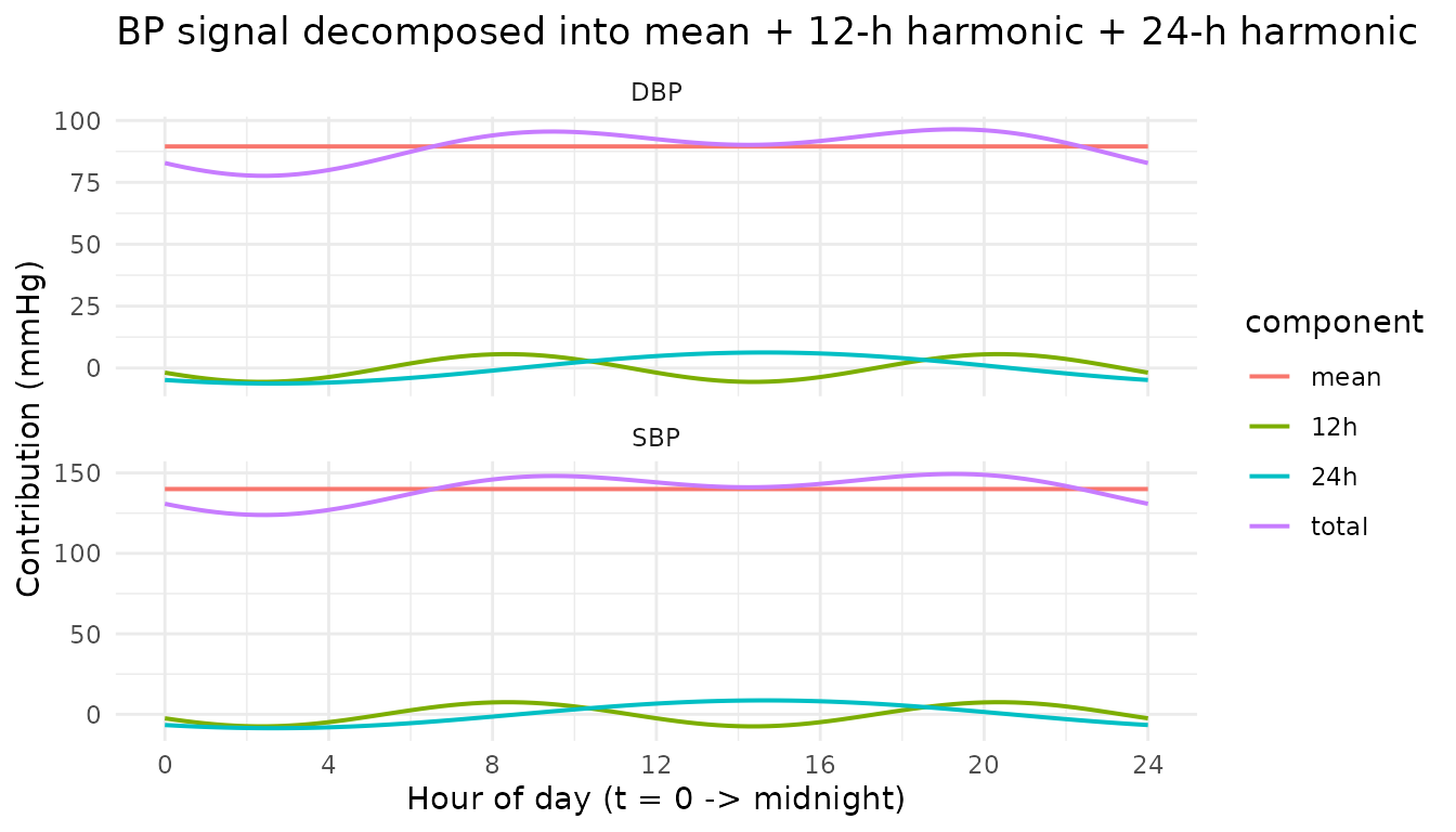
Per-harmonic decomposition of the typical-value BP signal. ‘mean’ is Base_k; ‘12-h’ is the A1k cosine term; ‘24-h’ is the A2k cosine term; ‘total’ sums all three.
Population VPC (replicates Sheng 2013 Figure 3 spread)
Sheng 2013 Figure 3 shows the 24-h ABPM VPC for each of the four studies with median and 2.5th-97.5th percentile bands. Reproduce the band shape on a simulated cohort matched to Study 1 (n = 38 subjects) using the IIV and additive residual error encoded in the model.
set.seed(20130617L)
n_sub <- 38L

# One sampling night per subject: 15-min grid 8 AM-10 PM, 30-min 10 PM-8 AM,
# replicated across two consecutive days so each subject contributes a full
# 24-h ABPM profile starting at midnight (t=0) of day 1.
ev_pop <- do.call(rbind, lapply(seq_len(n_sub), function(i) {
  day_grid   <- seq(8/24, 22/24, by = 0.25/24)         # 8 AM-10 PM, 15 min
  night_grid <- c(seq(22/24, 1, by = 0.5/24), seq(0, 8/24, by = 0.5/24))  # 10 PM-8 AM, 30 min
  data.frame(
    id    = i,
    time  = sort(unique(c(day_grid, night_grid))),
    amt   = 0,
    evid  = 0L
  )
}))

sim_pop <- rxode2::rxSolve(mod, events = ev_pop, returnType = "data.frame")
sim_pop$hour <- sim_pop$time * 24
vpc_long <- sim_pop |>
  dplyr::select(hour, SBP, DBP, sim) |>
  tidyr::pivot_longer(c(SBP, DBP), names_to = "output", values_to = "BP")

vpc_summary <- vpc_long |>
  dplyr::mutate(hour_bin = floor(hour)) |>
  dplyr::group_by(hour_bin, output) |>
  dplyr::summarise(
    Q025 = stats::quantile(BP, 0.025, na.rm = TRUE),
    Q50  = stats::quantile(BP, 0.50,  na.rm = TRUE),
    Q975 = stats::quantile(BP, 0.975, na.rm = TRUE),
    .groups = "drop"
  )

ggplot(vpc_summary, aes(hour_bin, Q50)) +
  geom_ribbon(aes(ymin = Q025, ymax = Q975), alpha = 0.25, fill = "#7f8c8d") +
  geom_line(linewidth = 0.7, colour = "#2c3e50") +
  facet_wrap(~ output, ncol = 1, scales = "free_y") +
  scale_x_continuous(breaks = seq(0, 24, by = 4)) +
  labs(x = "Hour of day",
       y = "Blood pressure (mmHg)",
       title = "VPC of simulated 24-h ABPM (Study 1 cohort, n = 38)",
       caption = "Median + 2.5th-97.5th band per hour bin. Replicates Sheng 2013 Figure 3 Study 1 panel.") +
  theme_minimal()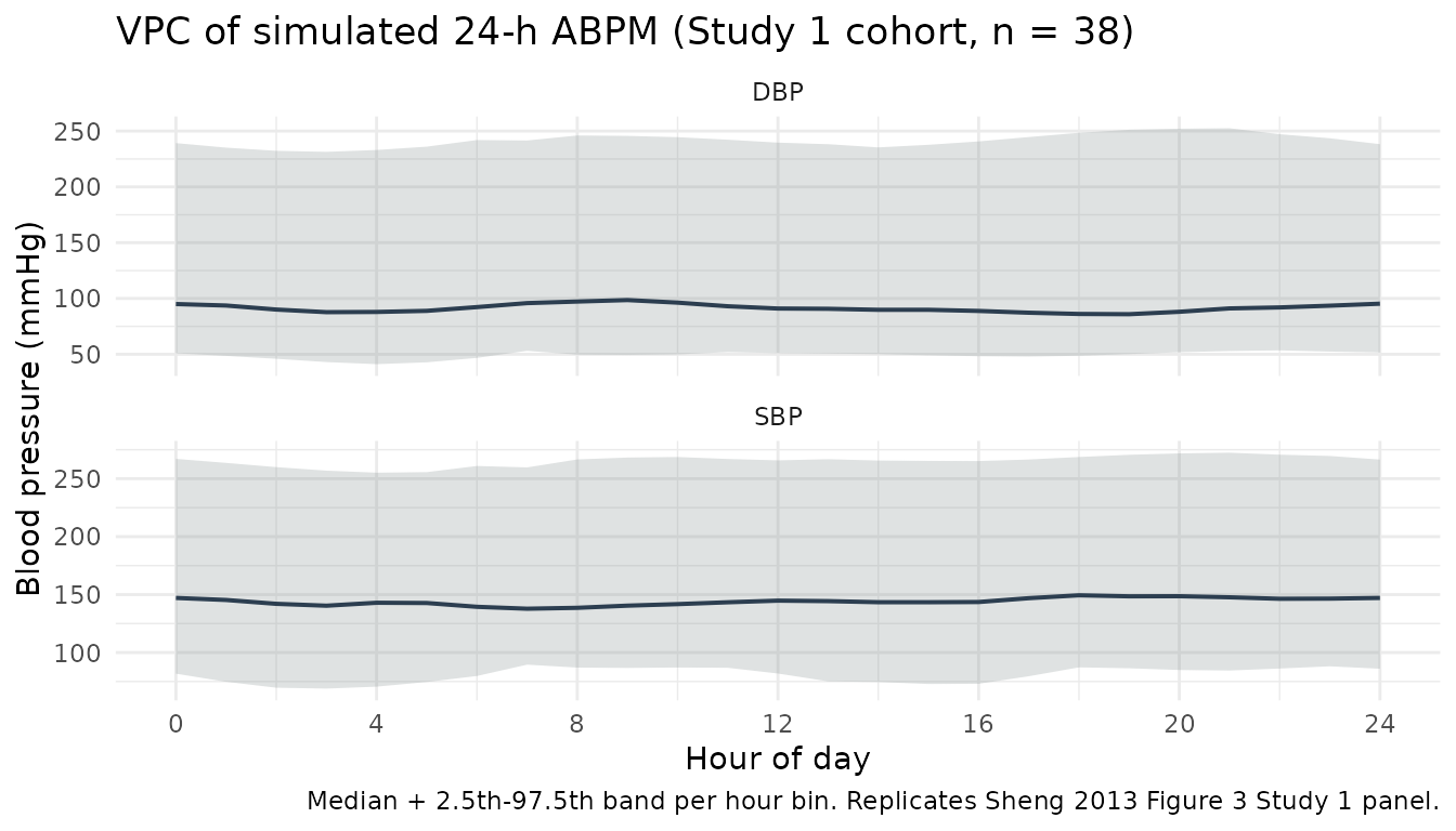
Population VPC of simulated SBP (top) and DBP (bottom) across 24 h. Median and 2.5th-97.5th percentile bands replicate the shape of Sheng 2013 Figure 3 (Study 1 panel).
knitr::kable(vpc_summary |>
               dplyr::filter(hour_bin %in% c(0, 6, 9, 14, 19, 22)),
             digits = 1,
caption = "VPC summary at selected canonical hours (median + 95% percentile band).")| hour_bin | output | Q025 | Q50 | Q975 |
|---|---|---|---|---|
| 0 | DBP | 50.9 | 95.0 | 239.2 |
| 0 | SBP | 81.8 | 147.1 | 267.1 |
| 6 | DBP | 46.7 | 92.3 | 242.0 |
| 6 | SBP | 79.8 | 139.4 | 261.0 |
| 9 | DBP | 49.4 | 98.6 | 245.7 |
| 9 | SBP | 86.7 | 140.4 | 268.2 |
| 14 | DBP | 50.1 | 89.8 | 235.4 |
| 14 | SBP | 74.5 | 143.4 | 265.7 |
| 19 | DBP | 50.1 | 85.9 | 251.2 |
| 19 | SBP | 86.4 | 148.5 | 270.6 |
| 22 | DBP | 53.5 | 92.0 | 247.2 |
| 22 | SBP | 86.2 | 146.4 | 270.7 |
Cross-study consistency (Sheng 2013 Table 3)
Sheng 2013 Table 3 reports that the same structural model fit to
Studies 2, 3, and 4 yields parameter estimates very close to Study 1.
The packaged model is parameterised against Study 1 only; for users who
want a different cohort, the Study 2-4 and pooled estimates from Table 3
can be substituted via ini().
table3 <- tibble::tribble(
  ~parameter, ~Study1, ~Study2, ~Study3, ~Study4, ~Overall_pooled,
  "Base_1 (mmHg)",   140,   144,   138,   136,   139,
  "Base_2 (mmHg)",   89.5,  91.7,  88.8,  88.5,  89.5,
  "A_11 (mmHg)",     7.52,  7.83,  6.07,  7.11,  7.20,
  "A_21 (mmHg)",     8.64,  9.76,  7.59,  10.8,  9.45,
  "A_12 (mmHg)",     5.61,  5.78,  4.41,  5.08,  5.22,
  "A_22 (mmHg)",     6.27,  6.39,  6.05,  7.16,  6.55,
  "PHS1 (day)",     -0.652, -2.18, -2.16,  0.84, -2.16,
  "PHS2 (day)",      3.61,  3.61,  3.58,  4.58,  3.59,
  "sigma SBP (mmHg)", 12.85, 12.8, 12.6, 11.3, 12.2,
  "sigma DBP (mmHg)",  9.11,  9.28,  9.74,  8.96, 9.23
)
knitr::kable(table3,
caption = "Sheng 2013 Tables 2-3: structural parameter estimates across the four study cohorts and the four-study pooled fit.")| parameter | Study1 | Study2 | Study3 | Study4 | Overall_pooled |
|---|---|---|---|---|---|
| Base_1 (mmHg) | 140.000 | 144.00 | 138.00 | 136.00 | 139.00 |
| Base_2 (mmHg) | 89.500 | 91.70 | 88.80 | 88.50 | 89.50 |
| A_11 (mmHg) | 7.520 | 7.83 | 6.07 | 7.11 | 7.20 |
| A_21 (mmHg) | 8.640 | 9.76 | 7.59 | 10.80 | 9.45 |
| A_12 (mmHg) | 5.610 | 5.78 | 4.41 | 5.08 | 5.22 |
| A_22 (mmHg) | 6.270 | 6.39 | 6.05 | 7.16 | 6.55 |
| PHS1 (day) | -0.652 | -2.18 | -2.16 | 0.84 | -2.16 |
| PHS2 (day) | 3.610 | 3.61 | 3.58 | 4.58 | 3.59 |
| sigma SBP (mmHg) | 12.850 | 12.80 | 12.60 | 11.30 | 12.20 |
| sigma DBP (mmHg) | 9.110 | 9.28 | 9.74 | 8.96 | 9.23 |
Assumptions and deviations
No drug input, no compartments. This model is a baseline-BP rhythm fit to placebo-period data. Combine with a drug PK/PD turnover or Emax model when simulating antihypertensive trials. The vignette validation here is the endogenous / circadian-rhythm equivalent of a PKNCA check: typical-value trajectory match against Figure 1, decomposition match against the Methods equation, and VPC band match against Figure 3.
No covariates retained. Sheng 2013 screened gender, age, weight, and BMI against all eight structural parameters and found none significantly improved the fit (Results, page 1046: “The covariates, including gender, age, weight and BMI, did not significantly increase the goodness of fit”). The four screened covariates are preserved in
covariatesDataExcludedfor provenance only.IIV parameterisation mixes log-normal and additive. Sheng 2013 (“Statistical models”, page 1045) states
P_i = P_tv * exp(eta_i)witheta_i ~ N(0, omega^2)for all parameters. The Table 2 omega values for the two baselines (0.079, 0.12) are interpretable as log-scale variances – giving CV approximately 29-35%, well within range of the bootstrap CIs the same table reports. The Table 2 omega values for the amplitudes (5.63, 4.73, 6.58, 6.71) and phase shifts (10.9, 1.24) are NOT interpretable as log-scale variances: a log-normal interpretation would imply CV > 100% for every amplitude (sqrt(exp(5.63) - 1) ~ 16.8 = 1680%), which is incompatible with the narrow bootstrap CIs the same table reports. The only interpretation consistent with both the point estimates and the bootstrap CIs is that the amplitude and phase-shift IIV is additive on the linear scale, i.e.P_i = P_tv + eta_iwithomega^2in the units of the parameter itself (mmHg^2 or day^2). The packaged model encodes the baselines as log-normal and the amplitudes / phase shifts as additive, matching the bootstrap CIs reported in Sheng 2013 Table 2.Phase-shift periodicity. Cosines are 2*pi-periodic, so any individual draw of PHS1 (period 0.5 day) or PHS2 (period 1 day) is mathematically valid – a 3.30-day SD on PHS1 (~6.6 periods) does not constrain the effective phase, only its representation. The packaged model reproduces the paper’s published omega^2 values verbatim and does not impose any modular reduction inside
model().-
Time origin. The paper does not state the calendar zero explicitly. The packaged model assumes
t = 0corresponds to midnight: the 24-h-harmonic peak att = PHS2 mod 1 ~ 0.61 day = 2:38 PMmatches the typical daytime BP activity peak, and the 12-h-harmonic peaks at `t = -0.152 day mod 0.5 day~ 8:21 AM
and~ 8:21 PMmatch the published "two peaks and a valley" pattern. Users who prefer a different zero (e.g. relative to wake-up time) can shifttime` in the event table accordingly. Residual error encoded as additive SD per output. Sheng 2013 reports
epsilon ~ N(0, sigma^2)in the Statistical models paragraph but the Table 2 column unit is “(mmHg)”. Encoded here as the additive SD per output via~ add(addSd_<output>), consistent with the (mmHg) units the row label declares.PHS1 95% CI sign anomaly in Table 2. The bootstrap 95% CI reported in Sheng 2013 Table 2 for PHS1 is “-0.668 to 0.862”, straddling zero and exceeding the period (0.5 day) of the 12-h harmonic. The point estimate (-0.652, SEM 1.3%) is precise; the wide bootstrap CI likely reflects the periodic identifiability of phase rather than a structural uncertainty. Recorded verbatim; not used as a constraint in the packaged model.