Postmenopausal BMD + repeated time-to-fracture (Plan 2012)
Source:vignettes/articles/Plan_2012_bmd_fracture.Rmd
Plan_2012_bmd_fracture.RmdModel and source
mod_fn <- readModelDb("Plan_2012_bmd_fracture")
mod <- mod_fn()- Citation: Plan EL, Baron KT, Gastonguay MR, French JL, Gillespie WR, Riggs MM. Bayesian Joint Modeling of Bone Mineral Density and Repeated Time-To-Fracture Event for Multiscale Bone Systems Model Extension. PAGE (Population Approach Group in Europe) 2012 conference poster. URL https://metrumrg.com/wp-content/uploads/2017/10/Riggs_PAGE2012.pdf (no DOI assigned; PAGE 2012 abstract IV-04). Piecewise-linear BMD structure cited from Greendale GA et al. J Bone Miner Res 2012 (poster reference [5]).
- Description: Bayesian joint disease-progression model linking postmenopausal bone mineral density (BMD) decline to a repeated time-to-fracture hazard, fit by Plan et al. (PAGE 2012 conference poster) to the 2005-2008 NHANES dataset (1605 postmenopausal women, 204 fracture events total; one femoral-neck BMD measure per subject and 0-5 fracture events each). The BMD time-course is piecewise linear in years since final menstrual period (FMP), with three annualized percent-change slopes: menopause transition (t in [-1, 2] yr), early postmenopausal (t in [2, 5] yr), and long-term post-FMP (t > 5 yr). The fracture hazard is exponential (Weibull shape alpha = 1 in the final model) with a BMD-centred log-linear modulation h(t) = exp(theta_h * (1 + theta_bmd * (BMD(t) - 0.8))). The cumulative-hazard ODE d/dt(cumhaz) <- h accumulates from t = 0 (FMP), and the survival probability sur = exp(-cumhaz) is exposed as a derived output. BMI, NHANES ethnicity, and age at FMP were carried as ‘centered covariate effects on all parameters’ in the source Bayesian fit but the per-parameter coefficient magnitudes are not reported in the poster; they are recorded in covariatesDataExcluded for provenance. See validation vignette Errata for the slope-unit interpretation: the printed source equation BMD(t) = b + sum(slope * piece) is additive in linear g/cm^2 only if the slopes are interpreted as %/yr-of-baseline (the Greendale 2012 convention cited as reference [5] in the poster); the model() block does the /100 conversion explicitly.
- Article (PAGE 2012 conference poster): https://metrumrg.com/wp-content/uploads/2017/10/Riggs_PAGE2012.pdf
Population
Plan 2012 fits the joint BMD + repeated-fracture model to the 2005-2008 National Health and Nutrition Examination Survey (NHANES) cycle, restricted to 1605 postmenopausal women. Each subject contributes a single femoral-neck BMD measurement (dual-energy X-ray absorptiometry) and 0-5 self-reported fracture events (204 fracture events across the cohort).
Mean current age at the NHANES examination is 63 years (95% interpercentile range 27-85). Mean age at the final menstrual period (FMP) is 45 years (95% interpercentile range 26-57). The poster does not retabulate the NHANES weight or race distributions; nationally representative NHANES 2005-2008 sample weights span Non-Hispanic White, Non-Hispanic Black, Mexican American, Other Hispanic, and Other Race / Multi-Racial.
The model uses years since FMP as its time axis: t = 0 is the
subject’s own FMP, and the population is observed at a range of post-FMP
times rather than at a common post-FMP cohort age. The full population
metadata is available via
readModelDb("Plan_2012_bmd_fracture")()$meta$population.
Source trace
The per-parameter origin is recorded as an in-file comment next to
each ini() entry in
inst/modeldb/therapeuticArea/Plan_2012_bmd_fracture.R. The
table below collects them for review.
| Equation / parameter | Value | Source location |
|---|---|---|
b_bmd (BMD intercept at t = -1 yr) |
0.84 g/cm^2 | Plan 2012 Results, ‘Structural parameter estimates’ (BMD panel). |
s_tr (transition slope, %/yr of baseline) |
-1.66 | Plan 2012 Results, ‘Structural parameter estimates’. |
s_po (postmenopausal slope, %/yr) |
-0.85 | Plan 2012 Results, ‘Structural parameter estimates’. |
s_fi (final slope, %/yr) |
-0.34 | Plan 2012 Results, ‘Structural parameter estimates’. |
theta_h (log baseline hazard at BMD = bmd_ref) |
-5.5 (95% CI -5.49 to -5.54) | Plan 2012 Figure 5 right-panel caption. |
theta_bmd (BMD effect on hazard) |
1.5 (95% CI 1.49-1.52) | Plan 2012 Figure 5 right-panel caption. |
bmd_ref (hazard-centring BMD, fixed) |
0.8 g/cm^2 | Plan 2012 Figure 4 caption (‘BMD = 0.8 g/cm^2, alpha = 1’). |
addSd (additive residual SD on BMD) |
0.131 g/cm^2 (95% CI 0.127-0.136) | Plan 2012 Results, BMD panel (‘sigma = 0.131’). |
| BMD piecewise-linear equation | BMD(t) = b + s_tr*t_{-1,2} + s_po*t_{2,5} + s_fi*t_{5,inf} |
Plan 2012 Methods, ‘Models’, BMD line; structural form cited from reference [5] (Greendale 2012, J Bone Miner Res). |
| Hazard equation | h(t) = exp(theta_h * (1 + theta_bmd * (BMD(t) - bmd_ref))) |
Plan 2012 Figure 5 right-panel caption. |
| Survival equation |
S(t) = exp(-(integral h(u) du from t_{j-1} to t_j)^alpha),
with alpha = 1 in final model |
Plan 2012 Methods, ‘Models’, Fracture-risk line; final-model alpha = 1 per Figure 4 caption. |
Virtual cohort
The published Figures 3, 5, and 7 of the poster show population
trajectories without individual-level data. The replication below uses a
single-cohort typical-value simulation (rxode2::zeroRe() so
the additive residual error is suppressed) and a 100-subject stochastic
simulation for the Figure 3 predictive distribution. The cap of 100
subjects per arm is well under the nlmixr2lib 200-per-arm vignette
ceiling and keeps the render fast.
set.seed(20120525)

n_typical <- 1L
n_stoch   <- 100L

# Typical-value events: a dense observation grid from FMP (t = 0) to 60 yr
# post-FMP. The simulation grid is uniform in time-since-FMP, matching the
# x-axis of Figures 3 and 7. Each event is observation-only (evid = 0),
# placed on the BMD output via `cmt` left unset (rxode2 records the
# algebraic observation at every time point).
ev_typical <- rxode2::et(seq(0, 60, by = 0.5))

# Stochastic-VPC events for Figure 3: 100 subjects observed on the same grid.
make_stoch_events <- function(n_sub, t_grid) {
  ev <- rxode2::et(t_grid) |> rxode2::et(id = seq_len(n_sub))
  ev
}
ev_stoch <- make_stoch_events(n_stoch, seq(0, 60, by = 1))
Simulation
# `mod` is already the rxUi object from the meta chunk above
# (readModelDb returns the model function; calling it returns the UI).

# Typical-value (zero residual error) trajectory: BMD piecewise-linear,
# cumulative hazard, and survival under the final hazard model.
mod_typical <- rxode2::zeroRe(mod)
#> Warning: No omega parameters in the model
sim_typical <- rxode2::rxSolve(mod_typical, events = ev_typical) |>
  as.data.frame()

# Stochastic 100-subject simulation including the additive BMD residual error.
sim_stoch <- rxode2::rxSolve(mod, events = ev_stoch) |>
  as.data.frame()
#> Warning: multi-subject simulation without without 'omega'
Replicate published figures
Figure 3: posterior predictive BMD trajectory
Plan 2012 Figure 3 shows the posterior predictive distribution of femoral-neck BMD as a function of years since FMP, with stratification by FMP age (panel 1: FMP age 20-42 yr; panel 2: FMP age 42-64 yr). The stochastic simulation below approximates the predictive band by overlaying 100 individual trajectories under the additive residual error model (no covariate effects, because the BMD-model covariate coefficients are not reported in the poster).
ggplot(sim_stoch, aes(time, sim, group = id)) +
  geom_line(alpha = 0.15, colour = "grey40") +
  geom_line(data = sim_typical, aes(time, BMD, group = NULL),
            colour = "firebrick", linewidth = 0.9) +
  labs(
    x        = "Years since FMP",
    y        = expression("BMD (g/cm"^2*")"),
    title    = "Figure 3 - BMD trajectory under the Plan 2012 piecewise-linear model",
    subtitle = "Grey: 100 subjects under additive residual error. Red: typical-value trajectory.",
    caption  = "Replicates Plan 2012 Figure 3 (without the FMP-age covariate stratification)."
  ) +
  theme_bw()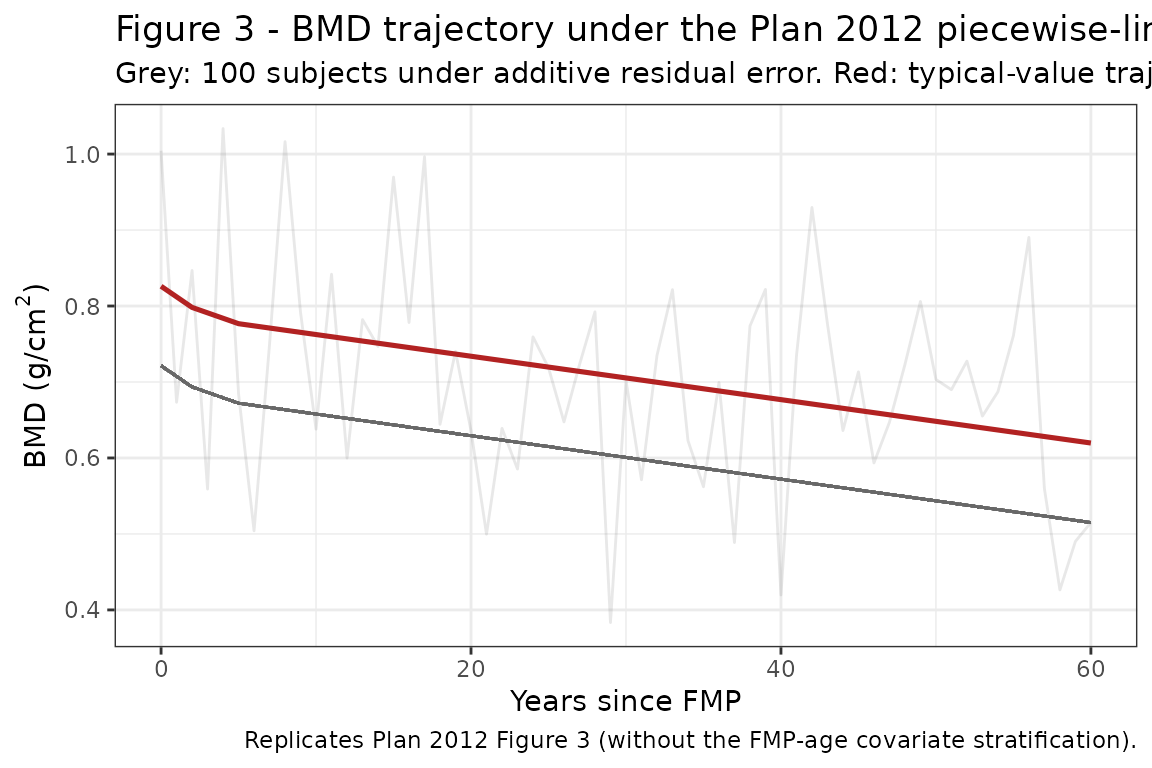
Replicates Figure 3 of Plan 2012 (population BMD time-course; covariates suppressed because per-parameter coefficients are not in the poster).
Figure 4: constant-hazard survival from FMP
For comparison, Plan 2012 Figure 4 shows the survival curve under a
constant (time-invariant) hazard fixed at
exp(theta_h) = exp(-5.5) ~ 4.1e-3 events/yr (the value of
the time-varying hazard at BMD = bmd_ref = 0.8 g/cm^2).
Below we reconstruct this constant-hazard reference by holding the
hazard constant at its t = 0 value.
h0     <- exp(-5.5)
t_grid <- sim_typical$time
sur_constant <- exp(-h0 * t_grid)

const_df <- data.frame(time = t_grid, sur = sur_constant)
ggplot(const_df, aes(time, sur)) +
  geom_line(colour = "steelblue", linewidth = 0.9) +
  scale_y_continuous(limits = c(0, 1)) +
  labs(
    x       = "Years since FMP",
    y       = "Proportion of fracture-free women",
    title   = "Figure 4 - Constant-hazard reference",
    caption = "Replicates Plan 2012 Figure 4 (h(t) fixed at exp(theta_h) = 0.00408 events/yr)."
  ) +
  theme_bw()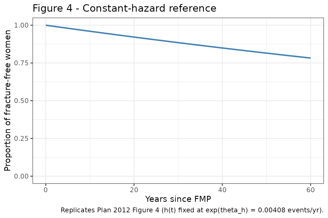
Replicates Figure 4 of Plan 2012 (constant-hazard survival from FMP).
Figure 5: final-model survival with BMD-driven time-varying hazard
Plan 2012 Figure 5 shows the same survival quantity under the final
model, in which the hazard is time-varying because BMD declines from b =
0.84 g/cm^2 at FMP through the piecewise-linear trajectory. The
implementation is the direct output of the cumhaz ODE
inside the packaged model.
ggplot(sim_typical, aes(time, sur)) +
  geom_line(colour = "darkorange3", linewidth = 0.9) +
  scale_y_continuous(limits = c(0, 1)) +
  labs(
    x       = "Years since FMP",
    y       = "Proportion of fracture-free women",
    title   = "Figure 5 - Final-model survival",
    caption = "Replicates Plan 2012 Figure 5 (h(t) = exp(theta_h * (1 + theta_bmd * (BMD(t) - 0.8))))."
  ) +
  theme_bw()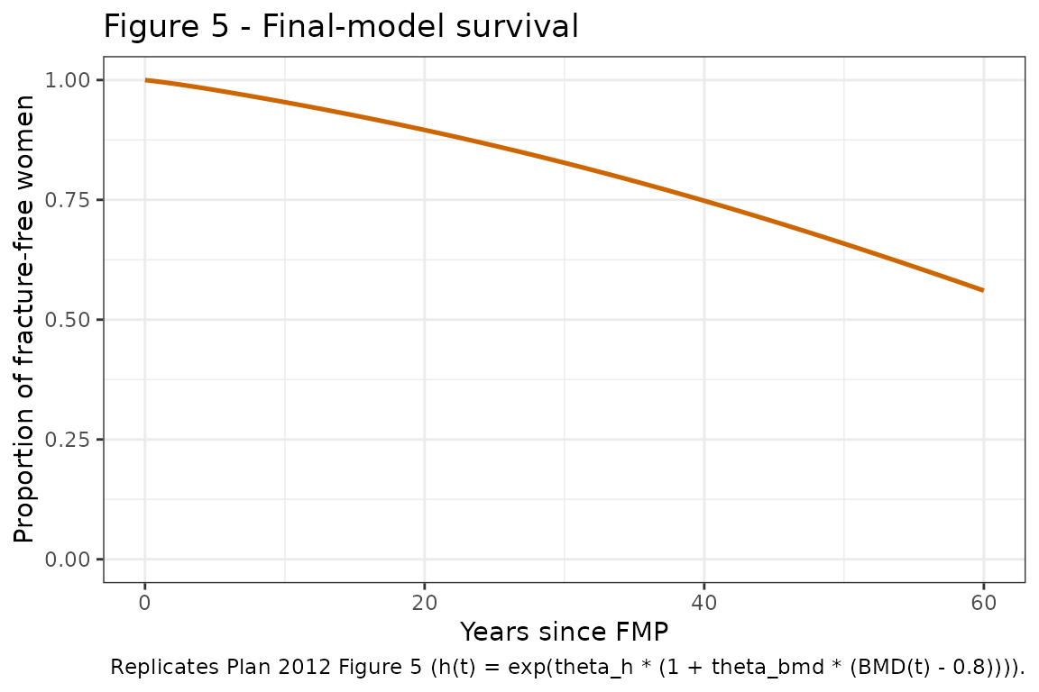
Replicates Figure 5 of Plan 2012 (final-model survival with time-varying hazard driven by BMD decline).
The fall in survival under the final model (Figure 5, ~0.56 at t = 60
yr) is steeper than under the constant-hazard reference (Figure 4, ~0.78
at t = 60 yr), reflecting the increased fracture risk that follows the
BMD decline. Plan 2012 reports a deltaDIC = 30 improvement
of the BMD-driven model over the constant-hazard model.
Figure 7: joint BMD + survival panel
Figure 7 of the poster overlays the typical-value BMD trajectory and the survival probability on a shared time axis. The packaged model exposes both quantities directly.
joint_df <- sim_typical |>
  dplyr::select(time, BMD, sur) |>
  tidyr::pivot_longer(c(BMD, sur), names_to = "panel", values_to = "value") |>
  dplyr::mutate(panel = factor(panel,
                               levels = c("BMD", "sur"),
                               labels = c("BMD (g/cm^2)",
                                          "Survival probability")))
ggplot(joint_df, aes(time, value)) +
  geom_line(colour = "darkgreen", linewidth = 0.9) +
  facet_wrap(~panel, scales = "free_y", ncol = 1) +
  labs(
    x       = "Years since FMP",
    y       = NULL,
    title   = "Figure 7 - Joint BMD and fracture-free probability",
    caption = "Replicates Plan 2012 Figure 7 (typical subject; covariates suppressed)."
  ) +
  theme_bw()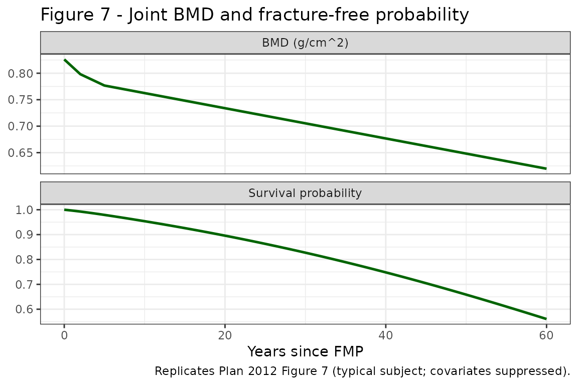
Replicates Figure 7 of Plan 2012 (joint BMD and fracture-free-probability trajectory for a typical postmenopausal subject starting at BMD ~ 0.83 g/cm^2 at FMP).
Comparison against published structural parameter estimates
The packaged model is parameter-identical to the published Plan 2012 final fit for the structural BMD and hazard parameters (the covariate effects and the per-subject random effects on BMD are not reported in the poster, so they are absent from the file).
publish <- tibble::tribble(
  ~parameter,  ~paper,          ~packaged,
  "b",         "0.84 g/cm^2",   "0.84",
  "s_tr",      "-1.66 %/yr",    "-1.66",
  "s_po",      "-0.85 %/yr",    "-0.85",
  "s_fi",      "-0.34 %/yr",    "-0.34",
  "theta_h",   "-5.5 (95% CI -5.49 to -5.54)", "-5.5",
  "theta_bmd", "1.5 (95% CI 1.49-1.52)",      "1.5",
  "BMDbar",    "0.8 g/cm^2 (fixed)",           "0.8 (fixed)",
  "alpha",     "1 (fixed; exponential RTTE)",  "1 (encoded as cumhaz ODE without alpha exponent)",
  "sigma",     "0.131 g/cm^2 (95% CI 0.127-0.136)", "0.131"
)
knitr::kable(publish,
             caption = "Published vs. packaged structural-parameter values.",
align = c("l", "l", "l"))| parameter | paper | packaged |
|---|---|---|
| b | 0.84 g/cm^2 | 0.84 |
| s_tr | -1.66 %/yr | -1.66 |
| s_po | -0.85 %/yr | -0.85 |
| s_fi | -0.34 %/yr | -0.34 |
| theta_h | -5.5 (95% CI -5.49 to -5.54) | -5.5 |
| theta_bmd | 1.5 (95% CI 1.49-1.52) | 1.5 |
| BMDbar | 0.8 g/cm^2 (fixed) | 0.8 (fixed) |
| alpha | 1 (fixed; exponential RTTE) | 1 (encoded as cumhaz ODE without alpha exponent) |
| sigma | 0.131 g/cm^2 (95% CI 0.127-0.136) | 0.131 |
Assumptions and deviations
-
Slope unit interpretation. The poster prints the
BMD model as
BMD(t) = b + s_tr*t_{-1,2} + s_po*t_{2,5} + s_fi*t_{5,inf}and reports slope values -1.66, -0.85, -0.34. Treated as additive in linear g/cm^2 these values give BMD(t = 60 yr) ~ -25 g/cm^2 (physically impossible). The poster cites Greendale 2012 (J Bone Miner Res, reference [5]) as the source of the piecewise-linear structure, and Greendale 2012 reports BMD slopes as annualized percent change of baseline BMD (%/yr). Under that convention, the packaged model applies the slopes asBMD(t) = b * (1 + sum(slope_k * piece_k) / 100), reproducing the ~ 0.84 -> 0.62 g/cm^2 decline shown in Figure 3 over t = 0 -> 60 yr post-FMP. The/100conversion happens inmodel()so theini()values match the poster’s reported numbers one-for-one. -
Covariate effects (BMI, NHANES ethnicity, age at FMP) absent
from forward simulation. The poster Methods section (‘Models’,
BMD line) states ‘Centered covariate effects added on all parameters’,
and the fracture-risk line lists ‘Investigated covariates: observed BMD,
BMD(t), FMPage, and time’. None of the per-parameter or per-hazard
covariate coefficient magnitudes are reported in the poster. The three
retained covariates are recorded in
covariatesDataExcludedfor provenance only; forward simulation reproduces the figure shapes without them. -
Combined IIV + RUV. Each subject contributes a
single femoral-neck BMD measurement, which precludes separating
between-subject variability from residual error. The reported
sigma = 0.131g/cm^2 is therefore encoded as the additive residual SD (addSd) and absorbs both IIV and RUV; no separateetalb_bmdis added. -
Weibull shape alpha not encoded as a primary
parameter. The poster’s Models section lists
alpha != 1as an investigated covariate but the final-model Figure 4 caption fixesalpha = 1(exponential RTTE between events). The packaged model encodes the cumulative-hazard ODE directly (d/dt(cumhaz) <- hazard) without exponentiating to alpha, equivalent to the alpha = 1 case. Adding a configurable alpha would require the RTTE simulation loop downstream of the cumhaz ODE. -
No explicit RTTE event-simulation hook. The
packaged model exposes
cumhazandsur = exp(-cumhaz)as derived outputs. Users who need to simulate the per-subject sequence of fracture event times follow the standard inverse-CDF approach: drawu ~ Uniform(0, 1), solvecumhaz(t_event) = -log(u)for the next event time, then resetcumhazto 0 and continue. This is intentionally left to the user so the model file stays compatible withrxode2::rxSolvefor both typical-value (Figure 5 / Figure 7) and stochastic (Figure 3) use cases. -
Hazard-model covariates (
observed BMD,BMD(t),FMPage,time) not all encoded. The packaged hazard usesBMD(t)(the time-varying BMD predicted by the piecewise-linear model) viatheta_bmd. The poster’s ‘Investigated covariates’ list also enumeratesobserved BMD(a time-fixed baseline observation) andFMPage; neither has a reported coefficient in the poster, and the right-panel caption of Figure 5 shows onlytheta_handtheta_bmd. The model therefore encodes only the BMD(t)-driven covariate effect.