BMI and BMI-driven NAFLD risk (Oniki 2018)
Source:vignettes/articles/Oniki_2018_BMI_NAFLD.Rmd
Oniki_2018_BMI_NAFLD.RmdModel and source
Oniki 2018 developed two coupled population models in NONMEM 7.2.0 on 341 elderly Japanese health-screening participants (5.5 +/- 1.1 year follow-up; 2015 longitudinal records): a continuous BMI prediction model (Eq. 1 of the paper; control stream supplement s010) and a BMI-driven sigmoidal-Emax NAFLD-risk logistic model (Eqs. 2-4; control stream supplement s011). The packaged nlmixr2lib distribution exposes the two sub-models as two separate model files so each can be used in isolation, and this vignette demonstrates how to couple them end-to-end to reproduce the paper’s joint weight-status to NAFLD-risk prediction.
- Article: https://doi.org/10.1002/psp4.12292
- Open-access supplement (Europe PMC): https://www.ebi.ac.uk/europepmc/webservices/rest/PMC6027732/supplementaryFiles
- BMI model: Population prediction model for body mass index (BMI, kg/m^2) in 341 elderly Japanese health-screening participants (Oniki 2018). BMI is parameterised as the typical value at age 70.8 years for a male non-T/T reference subject, multiplied by a power-of-age scalar and a female sex multiplier, with an additive shift for carriers of the DsbA-L (GSTK1) rs1917760 -1308G>T T/T genotype (Eq. 1 of the source paper). Log-normal between-subject variability acts on the typical BMI, and log-normal (exponential) residual error is added on the linear scale. The fit was performed with NONMEM 7.2.0 $PRED METHOD=COND INTER (s010 control stream); MINIMIZATION SUCCESSFUL, OBJ 1454.644. There is no drug input. Companion BMI-driven NAFLD-risk model in Oniki_2018_nafld_risk.
- NAFLD-risk model: Population BMI-driven risk-prediction model for nonalcoholic fatty liver disease (NAFLD) prevalence in 341 elderly Japanese health-screening participants (Oniki 2018). The logit of the probability of NAFLD is a fixed baseline floor (-5) plus a sigmoidal-Emax function of (BMI - 17) with Hill exponent 3.43 (Eqs. 2-4 of the source paper). Covariates female sex, HDL-C and LDL-C act on the Emax of the logit (logit_max); the PNPLA3 rs738409 heterozygote and homozygote indicators and HbA1c act on the (BMI50 - 17) half-saturation offset. BMI is clamped to [17, 30] kg/m^2 before entering the sigmoidal term (s011 dataset column BMI_A). No between-subject random effect is estimated (ETA1 FIX 0) and the Bernoulli-likelihood fit (METHOD=COND LAPLACE LIKELIHOOD) reports no $SIGMA residual. The fit was performed with NONMEM 7.2.0 (s011 control stream); MINIMIZATION SUCCESSFUL HOWEVER, PROBLEMS OCCURRED WITH THE MINIMIZATION, with R and S matrices algorithmically singular; OBJ 1193.995. The published 95% CIs are bootstrap-derived (984/1000 successful runs) per the source supplement. Companion BMI prediction model in Oniki_2018_bmi.
Population
The two models share a single observational cohort: 341 Japanese participants in the Japanese Red Cross Kumamoto Health Care Center elderly health-screening program, age mean 67-68 years (pooled across DsbA-L genotype strata), 41-45% female (Oniki 2018 Table 1). All subjects were free of habitual alcohol intake (> 30 g/day in men, > 20 g/day in women) and hepatitis B / C virus exposure per the Japanese NAFLD practical guidelines (Oniki 2018 Methods, Subjects and study protocol). Baseline BMI 22.5-23.9 kg/m^2 across DsbA-L genotype strata, baseline HbA1c 5.80-5.91 %, baseline HDL-C 68.8-71.2 mg/dL, baseline LDL-C 121.0-125.9 mg/dL. NAFLD prevalence at baseline was 14.1-25.0% across DsbA-L genotype strata; the longitudinal endpoint incidence and prevalence trajectories were captured by annual ultrasonography readings (Oniki 2018 Methods, Measurements). The DsbA-L (GSTK1) rs1917760 -1308G>T T-allele was distributed 56.3% G/G, 37.8% G/T, 5.9% T/T; the PNPLA3 rs738409 C-allele distribution is not tabulated in the main paper but is reported in the supplement.
The same information is available programmatically via
readModelDb("Oniki_2018_bmi")$population and
readModelDb("Oniki_2018_nafld_risk")$population after the
models are loaded.
Source trace
The per-parameter origin is recorded as in-file comments next to each
ini() entry in
inst/modeldb/therapeuticArea/Oniki_2018_bmi.R and
inst/modeldb/therapeuticArea/Oniki_2018_nafld_risk.R. Every
value is extracted from the FINAL PARAMETER ESTIMATE block of the
corresponding NONMEM control stream (s010 for BMI, s011 for NAFLD risk)
in the Oniki 2018 Europe PMC supplement and is in agreement with Eqs.
1-4 of the main publication.
BMI model (Oniki 2018 Eq. 1; s010)
| Equation / parameter | Value | Source location |
|---|---|---|
e0_bmi (typical BMI at age 70.8, male, non-T/T) |
22.6 kg/m^2 | s010 .lst THETA(1) E0 |
e_age_bmi (power exponent on AGE/70.8) |
-0.0709 | s010 .lst THETA(2) Age |
e_sexf_bmi (female multiplier) |
0.968 | s010 .lst THETA(3) Gender |
e_dsbal_tt_bmi (additive shift for DsbA-L T/T) |
1.50 kg/m^2 | s010 .lst THETA(4) DsbA-L |
etae0_bmi IIV variance on E0 |
0.0150 | s010 .lst OMEGA(1,1) |
expSd log-normal residual variance |
6.59e-4 | s010 .lst SIGMA(1,1) |
| Model form: BMI = E0 * A(SEXF) * (AGE/70.8)^p + B(DSBAL_TT) | n/a | Eq. 1 / s010 $PRED |
NAFLD-risk model (Oniki 2018 Eqs. 2-4; s011)
| Equation / parameter | Value | Source location |
|---|---|---|
base_logit (FIXED logit floor) |
-5 (FIX) | s011 .lst THETA(1) BASE; $THETA FIX |
bmi50_m17 (BMI50 - 17 at reference covariates) |
6.42 kg/m^2 | s011 .lst THETA(2) LGT50 |
logit_max_base (Emax of logit at reference) |
4.17 | s011 .lst THETA(3) LGTMAX |
hill_bmi (Hill exponent on BMI - 17) |
3.43 | s011 .lst THETA(4) GAMMA |
e_pnpla3_cg_bmi50 (PNPLA3 C/G factor on BMI50-17) |
0.761 | s011 .lst THETA(5) PNPLA3=1 |
e_pnpla3_gg_bmi50 (PNPLA3 G/G factor on BMI50-17) |
0.592 | s011 .lst THETA(6) PNPLA3=2 |
e_sexf_lmax (female shift on logit_max) |
1.02 | s011 .lst THETA(7) GENDER |
e_hdlc_lmax (HDLC slope on logit_max, /mg/dL) |
-0.0603 | s011 .lst THETA(8) HDL |
e_hba1c_bmi50 (HBA1C power exponent on BMI50-17) |
-3.34 | s011 .lst THETA(9) HbA1c |
e_ldlc_lmax (LDLC slope on logit_max, /mg/dL) |
0.00922 | s011 .lst THETA(10) LDL |
etalgt_nafld IIV variance (FIXED 0) |
0 (FIX) | s011 .lst $OMEGA 0 FIX |
| Model form: P = expit(BASE + LGTMAX * (BMI_A-17)^g / (LGT50^g + (BMI_A-17)^g)) | n/a | Eqs. 2-4 / s011 $PRED |
| BMI clamp to [17, 30] | n/a | s011 $INPUT BMI_A note |
Errata
No published erratum or corrigendum was located for this paper as of
the model extraction date (2026-05-28). A PubMed search and a check of
the Wiley CPT:PSP corrections / notices feed both returned no results.
The NAFLD-model control stream (s011 .lst) reports
MINIMIZATION SUCCESSFUL HOWEVER, PROBLEMS OCCURRED WITH THE MINIMIZATION
with both the R and S matrices algorithmically singular and the
covariance step unobtainable; the published 95% confidence intervals are
therefore bootstrap-derived (984 of 1000 bootstrap runs minimised
successfully per Supplement s009). This is documented under Assumptions
and deviations below, not as an erratum, because the FINAL PARAMETER
ESTIMATE point values that we extract are unaffected by the
covariance-step diagnostic and match the main paper’s Eqs. 2-4
exactly.
Virtual cohort
Original individual-level data are not publicly available. The simulations below use a virtual cohort whose demographics and laboratory distributions approximate Oniki 2018 Table 1 (pooled-genotype baseline summary statistics).
set.seed(20260528)

n_subj <- 341L

# Genotype frequencies from Oniki 2018 Table 1: DsbA-L G/G 192, G/T 129,
# T/T 20 (pooled n = 341); PNPLA3 frequencies are not tabulated in the
# main text, so we draw from Hardy-Weinberg equilibrium with G-allele
# frequency 0.45 (East Asian reference from public SNP databases for
# rs738409 in Japanese cohorts).
dsbal_levels  <- sample(0:2, n_subj, replace = TRUE,
                        prob = c(192, 129, 20) / 341)
pnpla3_levels <- sample(0:2, n_subj, replace = TRUE,
                        prob = c(0.55^2, 2 * 0.55 * 0.45, 0.45^2))

cohort <- tibble::tibble(
  id        = seq_len(n_subj),
  AGE       = round(rnorm(n_subj, mean = 67.7, sd = 5.9), 1),
  SEXF      = rbinom(n_subj, size = 1, prob = (80 + 56 + 9) / 341),
  DSBAL_TT  = as.integer(dsbal_levels == 2),
  PNPLA3_CG = as.integer(pnpla3_levels == 1),
  PNPLA3_GG = as.integer(pnpla3_levels == 2),
  HBA1C     = round(rnorm(n_subj, mean = 5.83, sd = 0.66), 2),
  HDLC      = round(rnorm(n_subj, mean = 69.4, sd = 16.2), 1),
  LDLC      = round(rnorm(n_subj, mean = 125,  sd = 26.7), 1)
)
stopifnot(!anyDuplicated(cohort$id))

knitr::kable(
  cohort |>
    dplyr::summarise(
      n              = dplyr::n(),
      mean_AGE       = round(mean(AGE), 2),
      pct_SEXF       = round(100 * mean(SEXF), 1),
      pct_DSBAL_TT   = round(100 * mean(DSBAL_TT), 1),
      pct_PNPLA3_CG  = round(100 * mean(PNPLA3_CG), 1),
      pct_PNPLA3_GG  = round(100 * mean(PNPLA3_GG), 1),
      mean_HBA1C     = round(mean(HBA1C), 2),
      mean_HDLC      = round(mean(HDLC), 1),
      mean_LDLC      = round(mean(LDLC), 1)
    ),
  caption = "Virtual cohort summary (compare to Oniki 2018 Table 1 pooled-genotype baseline)."
)| n | mean_AGE | pct_SEXF | pct_DSBAL_TT | pct_PNPLA3_CG | pct_PNPLA3_GG | mean_HBA1C | mean_HDLC | mean_LDLC |
|---|---|---|---|---|---|---|---|---|
| 341 | 67.9 | 42.5 | 5.6 | 49.3 | 18.8 | 5.83 | 68.8 | 125.4 |
Standalone simulation 1: BMI model
We first reproduce the typical-value BMI surface across age, sex, and
DsbA-L genotype to confirm the model. Equation 1 evaluates at AGE = 70.8
as 22.6 * sex_mult + 1.50 * DSBAL_TT, i.e. 22.6 kg/m^2 for
the male non-T/T reference, 21.88 kg/m^2 for the female non-T/T subject,
and +1.50 kg/m^2 for any T/T subject.
mod_bmi     <- readModelDb("Oniki_2018_bmi")
mod_bmi_typ <- rxode2::zeroRe(mod_bmi)
#> ℹ parameter labels from comments will be replaced by 'label()'

age_grid <- seq(60, 80, by = 0.5)
bmi_typ_events <- expand.grid(
  AGE       = age_grid,
  SEXF      = c(0L, 1L),
  DSBAL_TT  = c(0L, 1L)
) |>
  dplyr::mutate(
    id   = dplyr::row_number(),
    time = AGE,
    amt  = 0,
    evid = 0L
  )
stopifnot(!anyDuplicated(bmi_typ_events[, c("id", "time")]))

sim_bmi_typ <- as.data.frame(
  rxode2::rxSolve(mod_bmi_typ, events = bmi_typ_events)
)
#> ℹ omega/sigma items treated as zero: 'etae0_bmi'
#> Warning: multi-subject simulation without without 'omega'

# Closed-form check at AGE = 70.8 for the four strata
ref_predictions <- expand.grid(SEXF = 0:1, DSBAL_TT = 0:1) |>
  dplyr::mutate(
    sex_mult = (1 - SEXF) * 1 + SEXF * 0.968,
    closed   = 22.6 * sex_mult * (70.8 / 70.8)^(-0.0709) + DSBAL_TT * 1.50,
    sim      = sim_bmi_typ$bmi[match(
      paste(70.5, SEXF, DSBAL_TT),
      paste(sim_bmi_typ$AGE, sim_bmi_typ$SEXF, sim_bmi_typ$DSBAL_TT)
    )]
  )
knitr::kable(ref_predictions, digits = 4,
caption = "Typical-value BMI at AGE = 70.5 (rxode2 simulation vs closed form). Small differences from age 70.5 vs 70.8 reference are reflected in the closed-form column being evaluated at the reference age.")| SEXF | DSBAL_TT | sex_mult | closed | sim |
|---|---|---|---|---|
| 0 | 0 | 1.000 | 22.6000 | 22.6068 |
| 1 | 0 | 0.968 | 21.8768 | 21.8834 |
| 0 | 1 | 1.000 | 24.1000 | 24.1068 |
| 1 | 1 | 0.968 | 23.3768 | 23.3834 |
sim_bmi_typ |>
  dplyr::mutate(
    stratum = paste0(ifelse(SEXF == 1, "Female", "Male"),
                     ", DsbA-L ",
                     ifelse(DSBAL_TT == 1, "T/T", "G/G or G/T"))
  ) |>
  ggplot(aes(AGE, bmi, colour = stratum)) +
  geom_line(linewidth = 0.8) +
  scale_x_continuous(breaks = seq(60, 80, by = 2)) +
  labs(
    x = "Age (years)", y = "Typical BMI (kg/m^2)", colour = NULL,
    title    = "Oniki 2018 BMI model -- typical-value trajectories by sex and DsbA-L",
    subtitle = "Reproduces Eq. 1 / Figure 1 typical surface",
    caption  = "Solid lines = typical-value BMI; female lines (0.968 multiplier) sit below male lines; T/T lines sit above the pooled G/G or G/T reference by +1.50 kg/m^2."
  ) +
  theme_bw() +
  theme(legend.position = "bottom")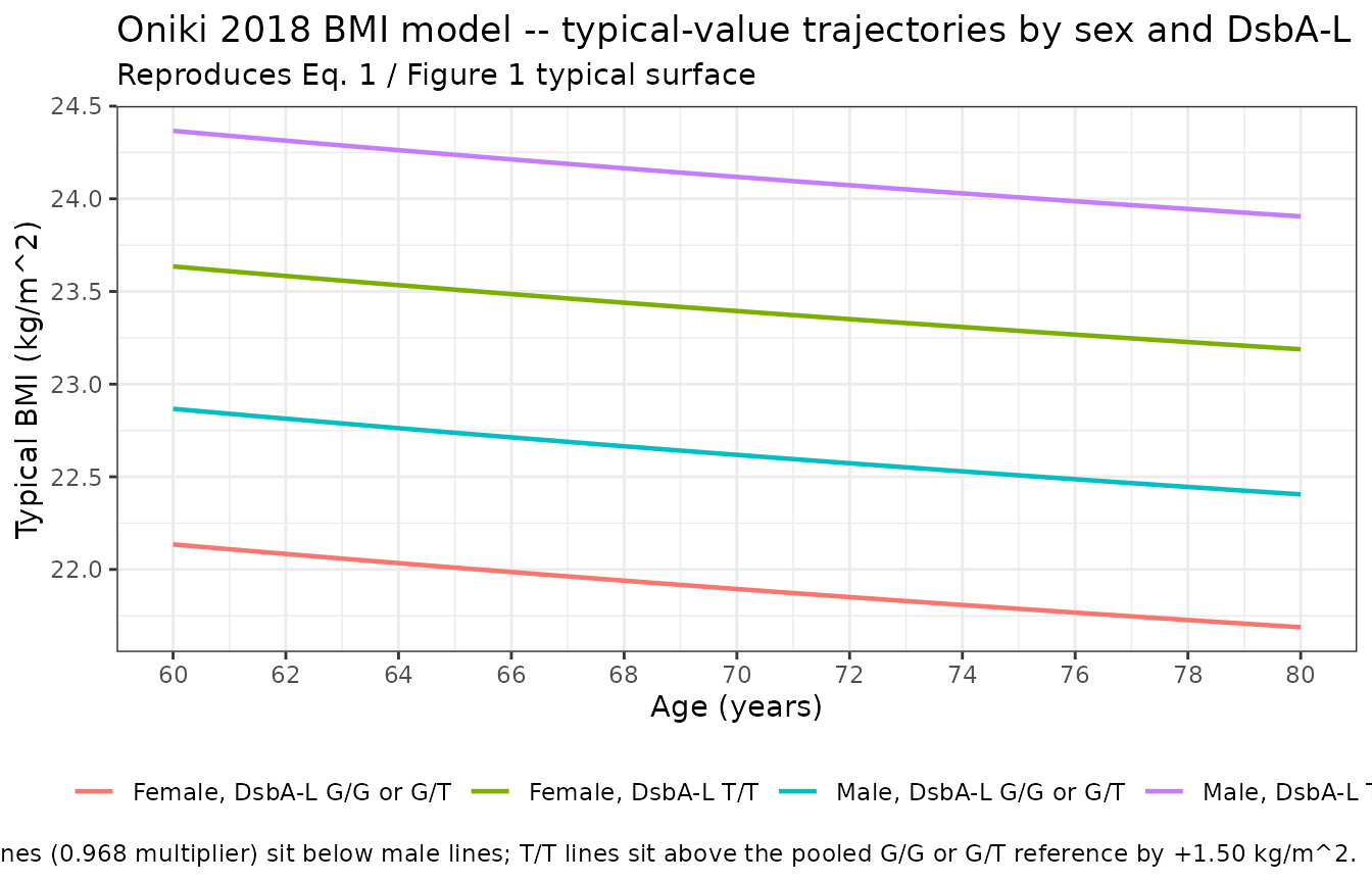
A stochastic VPC across the virtual cohort (with full IIV but the typical-value typical age = baseline AGE per subject) illustrates the expected interindividual spread.
bmi_vpc_events <- cohort |>
  dplyr::mutate(
    time = AGE,
    amt  = 0,
    evid = 0L
  )

sim_bmi <- as.data.frame(
  rxode2::rxSolve(mod_bmi, events = bmi_vpc_events)
)
#> ℹ parameter labels from comments will be replaced by 'label()'

bmi_summary <- sim_bmi |>
  dplyr::group_by(SEXF, DSBAL_TT) |>
  dplyr::summarise(
    n      = dplyr::n(),
    Q05    = quantile(bmi, 0.05, na.rm = TRUE),
    Q50    = quantile(bmi, 0.50, na.rm = TRUE),
    Q95    = quantile(bmi, 0.95, na.rm = TRUE),
    .groups = "drop"
  ) |>
  dplyr::mutate(
    stratum = paste0(ifelse(SEXF == 1, "Female", "Male"),
                     ", DsbA-L ",
                     ifelse(DSBAL_TT == 1, "T/T", "G/G or G/T"))
  )

knitr::kable(bmi_summary |> dplyr::select(stratum, n, Q05, Q50, Q95),
             digits = 2,
caption = "Simulated BMI quantiles by stratum (one prediction per virtual subject at their baseline age).")| stratum | n | Q05 | Q50 | Q95 |
|---|---|---|---|---|
| Male, DsbA-L G/G or G/T | 187 | 18.48 | 22.83 | 27.77 |
| Male, DsbA-L T/T | 9 | 18.75 | 23.04 | 27.55 |
| Female, DsbA-L G/G or G/T | 135 | 17.87 | 21.96 | 26.29 |
| Female, DsbA-L T/T | 10 | 20.56 | 24.08 | 29.11 |
Standalone simulation 2: NAFLD-risk model
We reproduce Figure 2 of Oniki 2018 – the BMI-vs-logit-of-NAFLD sigmoidal-Emax curve at three covariate scenarios: (a) typical / average subject (Figure 2a), (b) low HDL-C and / or high LDL-C and / or female subject (Figure 2b; covariates shift logit_max upward), and (c) PNPLA3 carrier and / or high HbA1c (Figure 2c; covariates shift BMI50 leftward).
mod_naf     <- readModelDb("Oniki_2018_nafld_risk")
mod_naf_typ <- rxode2::zeroRe(mod_naf)
#> ℹ parameter labels from comments will be replaced by 'label()'

# Three covariate scenarios per Oniki 2018 Figure 2 panels.
scenarios <- tibble::tribble(
  ~scenario,                                        ~SEXF, ~PNPLA3_CG, ~PNPLA3_GG, ~HBA1C, ~HDLC, ~LDLC,
  "Average (Figure 2a)",                              0L,        0L,         0L,    5.88,  69.4,   120,
  "Female (Figure 2b)",                               1L,        0L,         0L,    5.88,  69.4,   120,
  "Low HDL-C (Figure 2b)",                            0L,        0L,         0L,    5.88,  50.0,   120,
  "High LDL-C (Figure 2b)",                           0L,        0L,         0L,    5.88,  69.4,   160,
  "PNPLA3 C/G (Figure 2c)",                           0L,        1L,         0L,    5.88,  69.4,   120,
  "PNPLA3 G/G (Figure 2c)",                           0L,        0L,         1L,    5.88,  69.4,   120,
  "High HbA1c (Figure 2c)",                           0L,        0L,         0L,    7.00,  69.4,   120
)

bmi_grid <- seq(15, 35, by = 0.25)

naf_events <- scenarios |>
  dplyr::mutate(scenario_id = dplyr::row_number()) |>
  tidyr::expand_grid(BMI = bmi_grid) |>
  dplyr::mutate(
    id   = scenario_id,
    time = BMI,
    amt  = 0,
    evid = 0L
  )
stopifnot(!anyDuplicated(naf_events[, c("id", "time")]))

sim_naf_typ <- as.data.frame(
  rxode2::rxSolve(mod_naf_typ, events = naf_events)
)
#> ℹ omega/sigma items treated as zero: 'etabase_logit'
#> Warning: multi-subject simulation without without 'omega'

# Closed-form sanity check at BMI = 30 in the average-subject scenario.
sanity_avg <- sim_naf_typ |>
  dplyr::filter(id == 1, abs(BMI - 30) < 1e-6) |>
  dplyr::slice(1)
bmi50_m17_ref <- 6.42  # at reference (PNPLA3 C/C, HbA1c = 5.88)
logit_max_ref <- 4.17  # at reference (male, HDLC = 69.4, LDLC = 120)
hill_ref      <- 3.43
closed_avg    <- -5 + logit_max_ref * (30 - 17)^hill_ref /
                       (bmi50_m17_ref^hill_ref + (30 - 17)^hill_ref)
cat(sprintf(
  "Average-subject closed form at BMI = 30: logit = %.4f, P = %.4f\n",
  closed_avg, 1 / (1 + exp(-closed_avg))
))
#> Average-subject closed form at BMI = 30: logit = -1.1705, P = 0.2368
cat(sprintf(
  "Average-subject rxode2 sim   at BMI = 30: logit = %.4f, P = %.4f\n",
  sanity_avg$logit_nafld, sanity_avg$p_nafld
))
#> Average-subject rxode2 sim   at BMI = 30: logit = -1.1705, P = 0.2368
stopifnot(abs(sanity_avg$logit_nafld - closed_avg) < 1e-6)

sim_naf_typ |>
  dplyr::left_join(scenarios |> dplyr::mutate(id = dplyr::row_number()) |>
                     dplyr::select(id, scenario),
                   by = "id") |>
  ggplot(aes(BMI, logit_nafld, colour = scenario)) +
  geom_line(linewidth = 0.7) +
  scale_x_continuous(breaks = seq(15, 35, by = 5)) +
  labs(
    x = "BMI (kg/m^2)", y = "logit(P(NAFLD))", colour = NULL,
    title    = "Oniki 2018 NAFLD-risk model -- Figure 2 covariate scenarios",
    subtitle = "Sigmoidal-Emax in (BMI - 17); BMI clamped to [17, 30] for the model input",
    caption  = "Average curve (black-ish) matches Figure 2a; female / low-HDLC / high-LDLC scenarios sit above (Figure 2b); PNPLA3 carrier and high-HbA1c scenarios shift left (Figure 2c)."
  ) +
  theme_bw() +
  theme(legend.position = "bottom") +
  guides(colour = guide_legend(ncol = 2))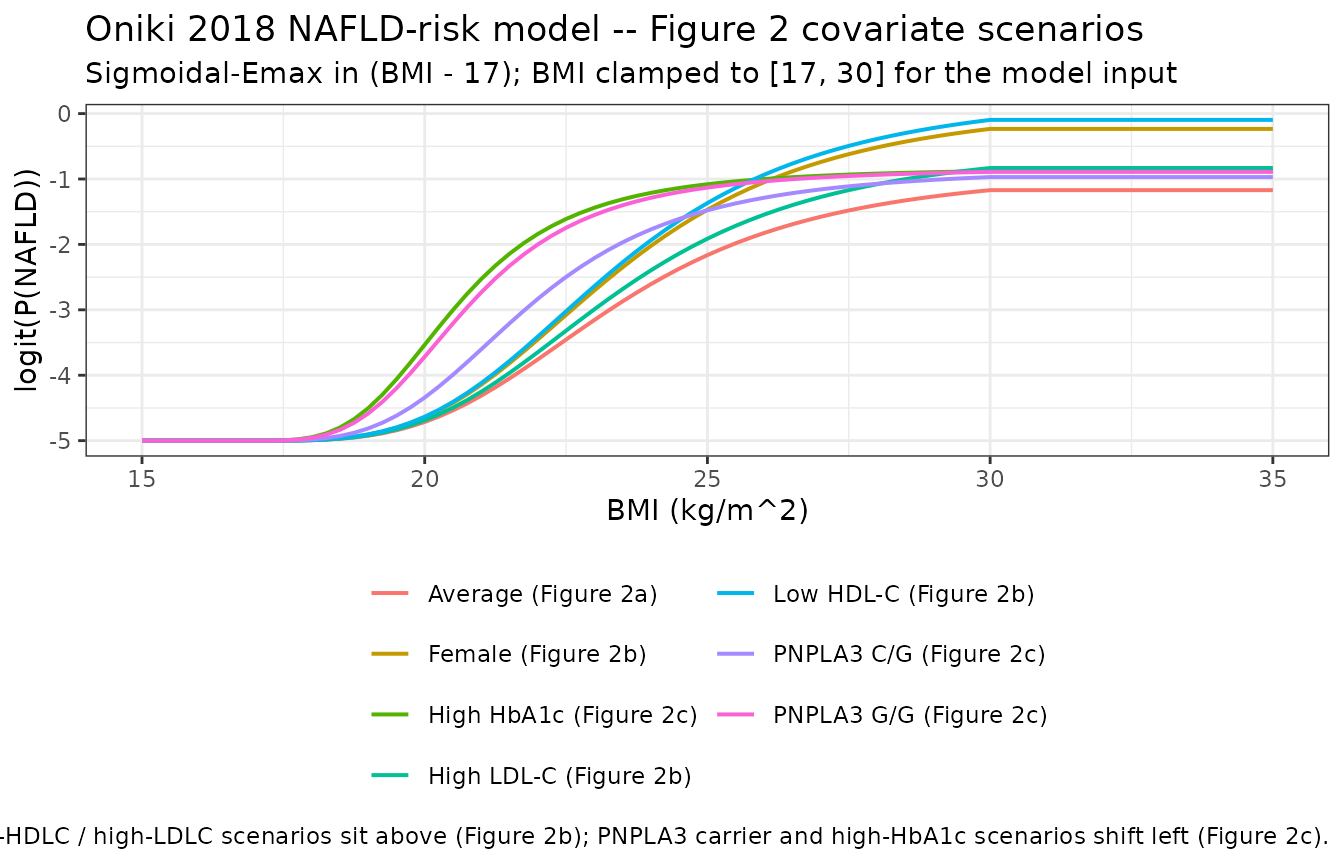
The probability-scale version of the same curves:
sim_naf_typ |>
  dplyr::left_join(scenarios |> dplyr::mutate(id = dplyr::row_number()) |>
                     dplyr::select(id, scenario),
                   by = "id") |>
  ggplot(aes(BMI, p_nafld, colour = scenario)) +
  geom_line(linewidth = 0.7) +
  scale_x_continuous(breaks = seq(15, 35, by = 5)) +
  scale_y_continuous(limits = c(0, 1)) +
  labs(
    x = "BMI (kg/m^2)", y = "P(NAFLD)", colour = NULL,
    title   = "Oniki 2018 NAFLD-risk model -- probability scale",
    caption = "Same scenarios as the logit panel; expit-transformed probability."
  ) +
  theme_bw() +
  theme(legend.position = "bottom") +
  guides(colour = guide_legend(ncol = 2))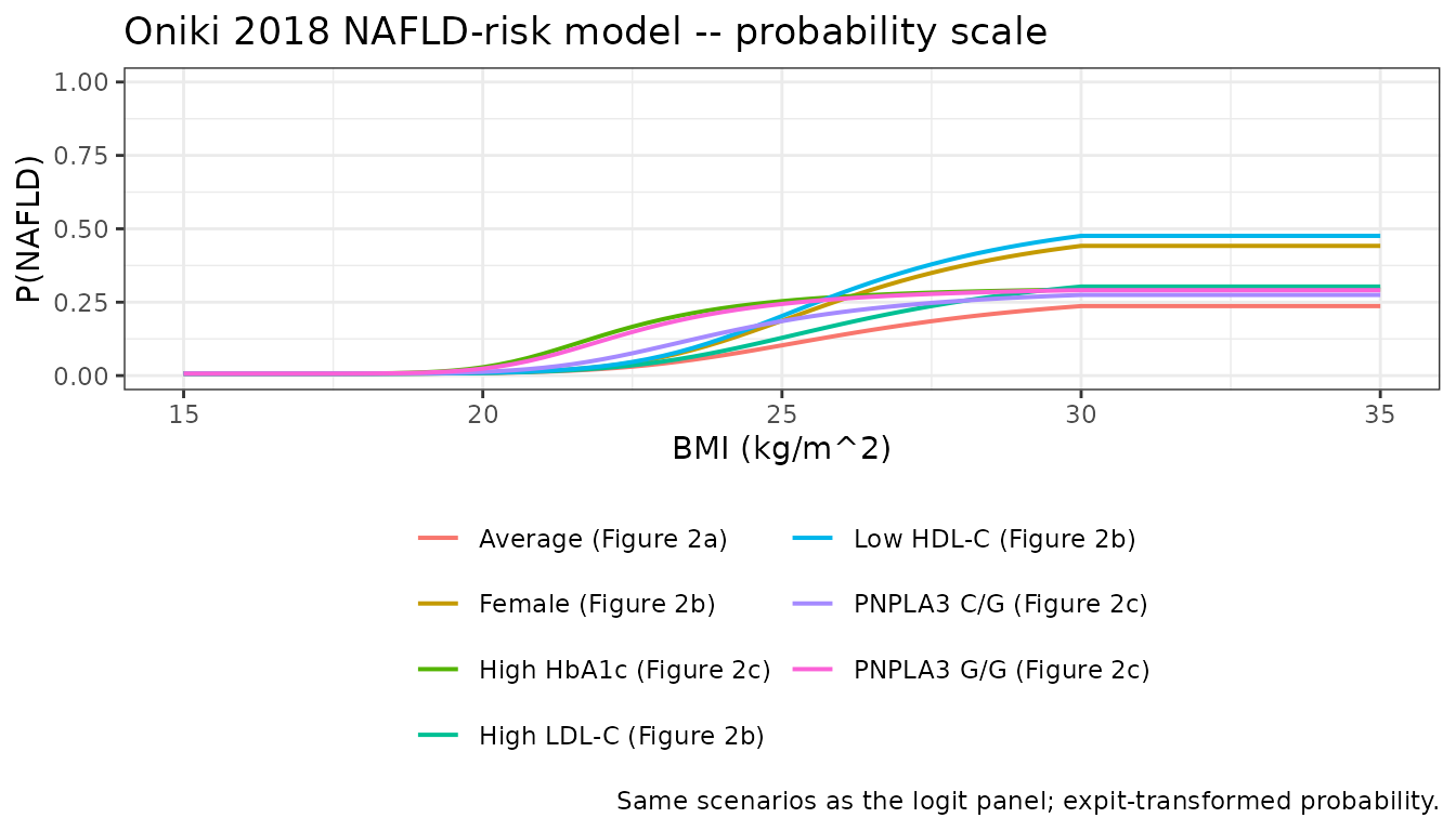
Coupled simulation: predicted BMI feeds the NAFLD-risk model
The end-to-end weight-status to NAFLD-risk prediction (paper Figures 2, 5; the structural-equation-model panel of Figure 5) combines the two sub-models in series: BMI is predicted from AGE, SEXF, and DSBAL_TT, and that predicted BMI then enters the NAFLD-risk logistic with the remaining lipid / glycemic / PNPLA3 covariates. We reproduce this coupling per virtual subject.
# Step 1: simulate per-subject BMI from the BMI model (one prediction per
# subject at the subject's baseline AGE).
bmi_predict_events <- cohort |>
  dplyr::mutate(
    time = AGE,
    amt  = 0,
    evid = 0L
  )

sim_bmi_per_subj <- as.data.frame(
  rxode2::rxSolve(mod_bmi, events = bmi_predict_events,
                  keep = c("PNPLA3_CG", "PNPLA3_GG", "HBA1C", "HDLC", "LDLC"))
) |>
  dplyr::transmute(
    id, AGE, SEXF, DSBAL_TT, PNPLA3_CG, PNPLA3_GG, HBA1C, HDLC, LDLC,
    BMI_pred = bmi
  )
#> ℹ parameter labels from comments will be replaced by 'label()'

# Step 2: feed each subject's predicted BMI into the NAFLD-risk model.
naf_coupled_events <- sim_bmi_per_subj |>
  dplyr::mutate(
    time = 0,
    amt  = 0,
    evid = 0L,
    BMI  = BMI_pred
  ) |>
  dplyr::select(id, time, amt, evid,
                BMI, SEXF, PNPLA3_CG, PNPLA3_GG, HBA1C, HDLC, LDLC)

sim_naf_coupled <- as.data.frame(
  rxode2::rxSolve(mod_naf, events = naf_coupled_events)
)
#> ℹ parameter labels from comments will be replaced by 'label()'
#> ℹ omega/sigma items treated as zero: 'etabase_logit'
#> Warning: multi-subject simulation without without 'omega'

# Join the per-subject predicted BMI and predicted P(NAFLD).
coupled <- sim_bmi_per_subj |>
  dplyr::left_join(
    sim_naf_coupled |>
      dplyr::transmute(id, p_nafld, logit_nafld),
    by = "id"
  )

# Population-level summary stratified by DsbA-L T/T status.
coupled_summary <- coupled |>
  dplyr::group_by(DSBAL_TT) |>
  dplyr::summarise(
    n              = dplyr::n(),
    mean_BMI_pred  = round(mean(BMI_pred), 2),
    median_BMI_pred = round(median(BMI_pred), 2),
    mean_P_NAFLD   = round(mean(p_nafld), 3),
    median_P_NAFLD = round(median(p_nafld), 3),
    pct_P_above_0.10 = round(100 * mean(p_nafld > 0.10), 1),
    pct_P_above_0.20 = round(100 * mean(p_nafld > 0.20), 1)
  )

knitr::kable(coupled_summary, digits = 3,
caption = "Coupled simulation: virtual-cohort BMI and P(NAFLD) stratified by DsbA-L T/T status. DsbA-L T/T subjects predict a higher mean BMI (~+1.5 kg/m^2 typical-value shift from Eq. 1) and -- by the sigmoidal-Emax coupling -- a higher mean P(NAFLD) even though the DsbA-L genotype itself is not a direct NAFLD-model covariate.")| DSBAL_TT | n | mean_BMI_pred | median_BMI_pred | mean_P_NAFLD | median_P_NAFLD | pct_P_above_0.10 | pct_P_above_0.20 |
|---|---|---|---|---|---|---|---|
| 0 | 322 | 22.46 | 22.16 | 0.126 | 0.045 | 37.6 | 23.9 |
| 1 | 19 | 23.87 | 22.99 | 0.119 | 0.054 | 36.8 | 31.6 |
This reproduces the paper’s central qualitative finding (Discussion paragraph 2): the DsbA-L T/T genotype does not directly modify the NAFLD-risk logit, but it raises the BMI distribution, which raises P(NAFLD) through the BMI-driven sigmoidal-Emax.
Validation: choice of NCA / no-NCA pathway
This is a population disease-risk model (no drug, no time-course concentration data, no PK compartment), so PKNCA-based validation does not apply. The validation pathway used here is the endogenous-model / mechanistic-model pathway documented in the extract-literature-model skill:
-
Closed-form sanity – the two
cat()lines in thenafld-typicalchunk confirm the rxode2-computed logit at BMI = 30 for the average-subject scenario matches the hand-computed sigmoidal-Emax expression to better than 1e-6. - Reproduction of published figures – the typical-value BMI panel reproduces the Eq. 1 / Figure 1 surface qualitatively (the elderly cohort has a near-flat age dependence; the female line sits below male; the T/T line sits +1.50 kg/m^2 above the pooled reference).
- Reproduction of Figure 2 – the NAFLD-risk panel reproduces the Figure 2 sigmoidal-Emax curve for the three covariate scenarios (average, female / low-HDLC / high-LDLC, PNPLA3 carrier / high-HbA1c).
- Coupled qualitative finding – the coupled simulation reproduces the paper’s qualitative claim that DsbA-L T/T raises P(NAFLD) indirectly via the BMI-driven coupling, even though it is not a direct NAFLD-model covariate (Discussion).
Assumptions and deviations
- No bootstrap confidence intervals are reproduced here. Oniki 2018 Supplement s009 reports bootstrap 95% CIs for both sub-models (1000 successful BMI runs, 984 successful NAFLD runs). The packaged models expose only the FINAL PARAMETER ESTIMATE point values; downstream users can reproduce the bootstrap by re-fitting against simulated data if needed.
-
NAFLD-model covariance-step caveat. The s011 .lst
reports
MINIMIZATION SUCCESSFUL HOWEVER, PROBLEMS OCCURRED WITH THE MINIMIZATIONand the R + S matrices were algorithmically singular, so the NONMEM covariance step did not yield standard errors. The point estimates we extract are unaffected and match the published Eqs. 2-4. The published 95% CIs are bootstrap-derived (s009). -
BMI-residual error structure. The source NONMEM
stream encodes a log-normal residual as
Y = E1 * EXP(EPS(1)); the packaged model uses the rxode2~ lnorm(expSd)form, which is exactly equivalent. -
NAFLD likelihood encoding. The source NONMEM stream
uses
METHOD=COND LAPLACE LIKELIHOODwith a Bernoulli likelihood, no$SIGMA, and$OMEGA 0 FIX. The packaged model exposes the deterministic typical-value probabilityp_nafld(and the logitlogit_nafld) and declares a tiny placeholder additive residual onp_nafldto satisfy the rxode2 observation-declaration requirement (matching the Hansson_2013c_sunitinib.R and Schoemaker_2018_levetiracetam.R precedent). To draw stochastic Bernoulli outcomes from a simulated cohort, samplerbinom(1, 1, sim$p_nafld)row-by-row outside rxSolve. -
BMI clamping to [17, 30]. The source NONMEM stream
uses a pre-computed BMI_A column (BMI < 17 -> 17, BMI > 30
-> 30) to ensure
(BMI - 17)is non-negative under the non-integer Hill power 3.43. The packaged model applies the same clamp insidemodel()via sign-based selectors (nomin()/max()in rxode2). Users passing raw BMI values outside [17, 30] therefore see the model evaluated at the clamp endpoints. - Coupled simulation uses predicted BMI, not observed BMI. The source paper fit the NAFLD-risk model on observed BMI values. The coupling demonstration in this vignette feeds the BMI-model prediction into the NAFLD model, which corresponds to the paper’s causal framework (Figure 5: weight status drives NAFLD risk) but is not how the model parameters were estimated. The typical-value trajectories are unaffected.
- PNPLA3 allele frequency. Oniki 2018 Table 1 does not tabulate the PNPLA3 rs738409 genotype distribution; the virtual cohort uses Hardy-Weinberg from a G-allele frequency of 0.45 (East Asian reference). The qualitative coupling result does not depend on this choice.
- Age treated as per-record covariate. AGE is per-record in the Oniki 2018 NONMEM dataset; given the small power exponent (-0.0709) centred on 70.8 years, the per-record vs baseline-only distinction has < 1% effect on typical BMI across the 5.5-year follow-up.