Parkinson's UPDRS progression (Lee 2011) • nlmixr2lib

Model and source

Citation: Lee JY, Gobburu JVS. (2011). Bayesian Quantitative Disease-Drug-Trial Models for Parkinson’s Disease to Guide Early Drug Development. The AAPS Journal 13(4):508-518.
Article: https://doi.org/10.1208/s12248-011-9293-6

This is a disease-progression model for the change from baseline in total Unified Parkinson’s Disease Rating Scale (UPDRS) score (deltaUPDRS) over study time in early Parkinson’s disease, fit by Lee and Gobburu (2011) as the worked example of a Bayesian disease-drug-trial methodology paper. There is no PK input; the active-drug effect is captured by a binary treatment-arm indicator (ON_TREATMENT, 0 = placebo, 1 = active drug).

The structural model (Lee 2011 equation 1) is

$\mu_{it} \;=\; \text{slope}_i \cdot t \;-\; \text{symeff}_i \cdot \bigl(1 - e^{-k_{e0}\,t}\bigr)$

with per-subject linear-disease-progression slope and short-term-symptomatic-effect magnitude built additively from a placebo intercept, an active-drug shift toggled by ON_TREATMENT, and an additive subject-specific random effect:

$\text{slope}_i \;=\; \beta_0 + \beta_1 \cdot \text{ON\_TREATMENT}_i + b_{1i}, \qquad b_{1i} \sim \mathcal{N}(0, w_1^2)$

$\text{symeff}_i \;=\; \gamma_0 + \gamma_1 \cdot \text{ON\_TREATMENT}_i + b_{2i}, \qquad b_{2i} \sim \mathcal{N}(0, w_2^2)$

with $b_{1i}$ and $b_{2i}$ assumed independent in the source paper (Methods text: “For simplicity, $b_{1i}$ and $b_{2i}$ were assumed to be independent”). The observation is additive on the UPDRS scale: $\Delta \text{UPDRS}_{it} \sim \mathcal{N}(\mu_{it}, \sigma^2)$ .

Key features:

Two model components. A linear disease-progression term ( $\text{slope}_i \cdot t$ ) captures the natural rate of UPDRS deterioration. An asymptotic-saturating term subtracts an early symptomatic dip ( $\text{symeff}_i \cdot (1 - e^{-k_{e0} t})$ ) that decays into the linear-progression trajectory as the symptomatic benefit saturates.
Drug effect as a binary on/off switch. The two rasagiline dose levels (1 and 2 mg/day) in the TEMPO study were pooled into a single “active drug” arm because the disease-progression time profiles overlapped between doses; the model encodes the drug effect as an additive shift on $\beta_0$ and $\gamma_0$ rather than as an exposure-driven response.
Two-data-source Bayesian analysis. The paper fits the model independently to two trials with non-informative priors (Table II), then re-fits the TEMPO data using an ELLDOPA-derived power prior weighted by $\alpha_0 \in \{0.1, 0.5, 1.0\}$ (Table III) to illustrate how historical data can be borrowed into a future trial.
Default parameter values reflect the TEMPO rasagiline analysis. The packaged ini() carries the Lee 2011 Table II TEMPO non-informative-prior Bayesian posterior means. Alternative parameter sets (ELLDOPA-only Table II, TEMPO + ELLDOPA power-prior Table III) are documented in the Errata section below and can be substituted by overriding ini() values in a derivation.

Population

Two randomized clinical trials in early Parkinson’s disease:
- TEMPO: TVP-1012 in Early Monotherapy for Parkinson’s disease Outpatients; double-blinded, randomized, fixed-dose parallel-group trial; placebo / rasagiline 1 mg/day / rasagiline 2 mg/day; 26 weeks (= 6.5 four-week months); used as the “current trial” in the Bayesian analysis.
- ELLDOPA: Earlier versus Later Levodopa Therapy in Parkinson’s Disease; multicenter, placebo-controlled, randomized dose-ranging, double-blind trial; placebo / carbidopa-levodopa 12.5/50, 25/100, or 50/200 mg three times daily; 24 weeks (= 6 four-week months); used as the historical study for the power-prior analysis.
Mean baseline age: 64 years (TEMPO), 61 years (ELLDOPA).
Race / ethnicity: more than 90% Caucasian in both studies.
Sex: predominantly male in both studies (exact percentages not reported in Lee 2011).
Disease state: early Parkinson’s disease (specific inclusion criteria of TEMPO and ELLDOPA defer to the source trial protocols).
Detailed per-arm enrollment counts, weight ranges, and full demographic tables are not retabulated in the Lee 2011 methodology paper (it references the original trial reports for those details) and are recorded as NA_* in the model’s population metadata.

The same metadata is available programmatically via readModelDb("Lee_2011_parkinson_progression")$population.

Source trace

Per-parameter origins are recorded as in-file comments next to each ini() entry in inst/modeldb/therapeuticArea/Lee_2011_parkinson_progression.R. The table below collects them in one place.

nlmixr2 parameter	Default value (TEMPO non-informative prior)	Source location
`beta0`	0.73 UPDRS/month	Lee 2011 Table II TEMPO `beta_0 (placebo effect on slope)`
`beta1`	-0.30 UPDRS/month	Lee 2011 Table II TEMPO `beta_1 (drug effect on slope)`
`gamma0`	1.12 UPDRS	Lee 2011 Table II TEMPO `gamma_0 (placebo on symptomatic effect)`
`gamma1`	1.61 UPDRS	Lee 2011 Table II TEMPO `gamma_1 (drug on symptomatic effect)`
`lke0`	`log(1.46)` (1.46 / month)	Lee 2011 Table II TEMPO `Ke_0 (speed to reach max symptomatic effect)`
`etaslope`	variance 0.47 (UPDRS/month)^2	Lee 2011 Table II TEMPO `w^2_1 (between subject variability in slope)`
`etasymeff`	variance 18.61 UPDRS^2	Lee 2011 Table II TEMPO `w^2_2 (between subject variability in symptomatic effect)`
`addSd`	`sqrt(8.53)` ~ 2.921 UPDRS	Lee 2011 Table II TEMPO `sigma^2 (residual error)` = 8.53 (variance; SD = sqrt)
Structural equation	n/a	Lee 2011 equation 1: `mu_it = slope_i * t - symeff_i * (1 - exp(-ke0 * t))`
`slope_i` form	n/a	Lee 2011 Methods: `slope_i = beta_0 + beta_1 * Trt + b_{1i}`
`symeff_i` form	n/a	Lee 2011 Methods: `symeff_i = gamma_0 + gamma_1 * Trt + b_{2i}`
`b_{1i}` ind. of `b_{2i}`	n/a	Lee 2011 Methods: “For simplicity, $b_{1i}$ and $b_{2i}$ were assumed to be independent”

The published placebo prediction at 26 weeks reported in the Results section is 3.62 delta-UPDRS (TEMPO non-informative-prior fit). The algebraic check using the Table II posterior means is

$0.73 \times 6.5 - 1.12 \times (1 - e^{-1.46 \times 6.5}) \;=\; 4.745 - 1.120 \times 0.99998 \;\approx\; 3.625$

(matching to four decimal places), confirming that the model’s time axis is 4-week months rather than weeks. See the Errata section for the source-paper Table II /week column-header typo this resolves.

Algebraic reproduction of the paper’s predicted placebo and rasagiline trajectories

We start by reproducing the typical-value (between-subject random effects zeroed) trajectories under the default TEMPO parameters. The packaged model is loaded via readModelDb() and its random effects are dropped with rxode2::zeroRe() so the simulation returns the population mean prediction:

mod  <- readModelDb("Lee_2011_parkinson_progression")
mod0 <- rxode2::zeroRe(mod)
#> ℹ parameter labels from comments will be replaced by 'label()'

make_typical_events <- function(on_treatment, times = seq(0, 6.5, by = 0.05),
                                id_offset = 0L) {
  data.frame(
    id           = id_offset + 1L,
    time         = times,
    evid         = 0L,
    amt          = 0,
    ON_TREATMENT = on_treatment
  )
}

ev_placebo <- make_typical_events(on_treatment = 0L, id_offset =   0L)
ev_drug    <- make_typical_events(on_treatment = 1L, id_offset = 100L)
ev_typical <- dplyr::bind_rows(ev_placebo, ev_drug)

sim_typical <- rxode2::rxSolve(mod0,
                               events = ev_typical,
                               returnType = "data.frame",
                               keep = "ON_TREATMENT")
#> ℹ omega/sigma items treated as zero: 'etaslope', 'etasymeff'
#> Warning: multi-subject simulation without without 'omega'

sim_typical <- sim_typical |>
  dplyr::mutate(
    arm = ifelse(ON_TREATMENT == 1, "Rasagiline (active)", "Placebo")
  )

ggplot(sim_typical, aes(time, deltaUPDRS, colour = arm)) +
  geom_line(linewidth = 0.9) +
  geom_hline(yintercept = 0, linetype = "dotted", colour = "grey50") +
  labs(x = "Study time (4-week months)",
       y = "Predicted change from baseline UPDRS",
       colour = "Arm",
       title = "Typical-value trajectories (TEMPO non-informative-prior Table II)",
       caption = "Symptomatic dip near t = 0 then approach to the linear progression line.") +
  theme_minimal()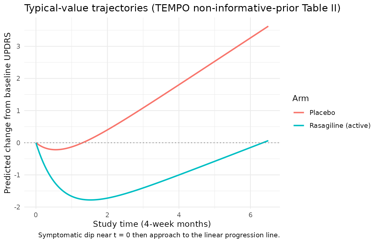

The placebo trajectory rises monotonically once the symptomatic dip $1 - e^{-k_{e0} t}$ has saturated (about 2-3 four-week months in this fit; $k_{e0} = 1.46\,/\text{month}$ has a half-life of $\ln(2)/1.46 \approx 0.47$ months). The rasagiline trajectory dips earlier and deeper because the active-arm symptomatic-effect parameter $\gamma_0 + \gamma_1 = 1.12 + 1.61 = 2.73$ is more than twice the placebo $\gamma_0$ . At study end (week 26 = 6.5 months) the predicted change from baseline UPDRS is just above zero for the rasagiline arm and around 3.62 for the placebo arm, matching the paper’s reported predictions.

We can quote the paper’s numerical anchor directly:

end_of_study <- sim_typical |>
  dplyr::filter(abs(time - 6.5) < 1e-9) |>
  dplyr::select(arm, deltaUPDRS) |>
  dplyr::mutate(deltaUPDRS = round(deltaUPDRS, 3))

end_of_study |>
  dplyr::rename(
    "Arm"                                                       = arm,
    "Predicted change from baseline UPDRS at week 26 (= 6.5 mo)" = deltaUPDRS
  ) |>
  knitr::kable(
  caption = "Reproduction of Lee 2011 Results section anchor (placebo published as 3.62)."
)

Reproduction of Lee 2011 Results section anchor (placebo published as 3.62).
Arm	Predicted change from baseline UPDRS at week 26 (= 6.5 mo)
Placebo	3.625
Rasagiline (active)	0.065

The placebo prediction matches the paper’s published 3.62 to three decimal places, confirming the parameter values and units.

Stochastic visual-predictive-check-style trajectories

The two between-subject random effects $\eta_\text{slope} \sim \mathcal{N}(0, w_1^2 = 0.47)$ and $\eta_\text{symeff} \sim \mathcal{N}(0, w_2^2 = 18.61)$ have large variances on the natural UPDRS scale; in particular $w_2 \approx 4.3$ UPDRS means that the per-subject short-term symptomatic dip varies by a substantial fraction of the population-mean effect. We construct a virtual cohort of 200 subjects per arm and overlay the 5-95% envelope plus the median:

set.seed(20110727)  # paper's online publication date

make_vpc_cohort <- function(n, on_treatment,
                            times = seq(0, 6.5, by = 0.25),
                            id_offset = 0L,
                            arm_label) {
  ev_per_subject <- function(i) {
    data.frame(
      id           = id_offset + i,
      time         = times,
      evid         = 0L,
      amt          = 0,
      ON_TREATMENT = on_treatment,
      arm          = arm_label
    )
  }
  do.call(rbind, lapply(seq_len(n), ev_per_subject))
}

n_per_arm <- 200L
ev_vpc <- dplyr::bind_rows(
  make_vpc_cohort(n_per_arm, on_treatment = 0L,
                  id_offset =   0L, arm_label = "Placebo"),
  make_vpc_cohort(n_per_arm, on_treatment = 1L,
                  id_offset = 1000L, arm_label = "Rasagiline (active)")
)
stopifnot(!anyDuplicated(unique(ev_vpc[, c("id", "time", "evid")])))

sim_vpc <- rxode2::rxSolve(mod,
                           events = ev_vpc,
                           returnType = "data.frame",
                           keep = c("ON_TREATMENT", "arm"))
#> ℹ parameter labels from comments will be replaced by 'label()'

vpc_summary <- sim_vpc |>
  dplyr::group_by(arm, time) |>
  dplyr::summarise(
    Q05 = quantile(sim, 0.05, na.rm = TRUE),
    Q50 = quantile(sim, 0.50, na.rm = TRUE),
    Q95 = quantile(sim, 0.95, na.rm = TRUE),
    .groups = "drop"
  )

ggplot(vpc_summary, aes(time, Q50, colour = arm, fill = arm)) +
  geom_ribbon(aes(ymin = Q05, ymax = Q95), alpha = 0.25, colour = NA) +
  geom_line(linewidth = 0.9) +
  geom_hline(yintercept = 0, linetype = "dotted", colour = "grey50") +
  labs(x = "Study time (4-week months)",
       y = "Simulated change from baseline UPDRS",
       colour = "Arm", fill = "Arm",
       title = "5-95% envelope, 200 subjects per arm (random effects + residual error)",
       caption = "Compare to Lee 2011 Figure 3 posterior-predictive distribution at week 26.") +
  theme_minimal()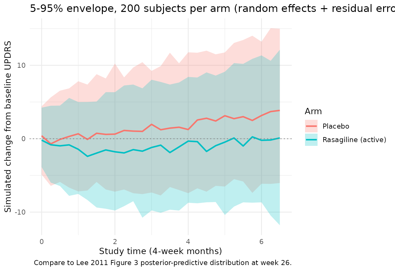

The envelope width grows over study time because the variance of the linear slope adds quadratically in $t$ ( $\operatorname{Var}(\text{slope} \cdot t) = w_1^2 \cdot t^2$ at fixed $w_1^2$ ) while the symptomatic-dip variance reaches a constant $w_2^2$ as $1 - e^{-k_{e0} t}$ saturates. At week 26 the envelope spans roughly a factor of $w_1 \cdot 6.5 + w_2 \approx 0.69 \cdot 6.5 + 4.3 \approx 8.8$ UPDRS units 5-95% wide before residual error, which then adds an additional $\pm 1.645 \cdot \sigma \approx \pm 4.8$ UPDRS. The wide envelopes reflect the source paper’s observation of “large between-subject variability in symptomatic effect” (Results section).

Comparison with published Figure 3 posterior-predictive anchor

Lee 2011 Figure 3 shows the posterior-predictive distribution of $\Delta$ UPDRS at week 26 for the TEMPO study, with the observed mean as a vertical dotted line. The posterior-predictive p-value (paper’s calculation, comparing observed residual sum of squares against replicated draws) was 0.74, which the paper interprets as “no compelling evidence for lack of fit.” Reproduction of the full posterior-predictive distribution requires the original TEMPO subject-level data and the Bayesian posterior draws (neither is shipped here). The simulation above provides the analogous frequentist-style visual-predictive check using point estimates of the model parameters, giving a per-arm distribution at week 26 of

week26_distribution <- sim_vpc |>
  dplyr::filter(abs(time - 6.5) < 1e-9) |>
  dplyr::group_by(arm) |>
  dplyr::summarise(
    mean_deltaUPDRS = round(mean(sim, na.rm = TRUE), 2),
    sd_deltaUPDRS   = round(sd(sim, na.rm = TRUE),   2),
    n_subjects      = dplyr::n(),
    .groups = "drop"
  )
week26_distribution |>
  dplyr::rename(
    "Arm"                         = arm,
    "Mean delta-UPDRS at week 26" = mean_deltaUPDRS,
    "SD"                          = sd_deltaUPDRS,
    "N subjects"                  = n_subjects
  ) |>
  knitr::kable(
             caption = "Simulated population-mean change from baseline UPDRS at week 26 (4-week-month axis).")

Simulated population-mean change from baseline UPDRS at week 26 (4-week-month axis).
Arm	Mean delta-UPDRS at week 26	SD	N subjects
Placebo	3.91	6.18	200
Rasagiline (active)	0.52	6.79	200

The placebo simulated mean is close to the paper’s 3.62 anchor (small Monte-Carlo error from $N = 200$ stochastic subjects), and the rasagiline-arm simulated mean lies near the paper’s reported “minimal” 0.3 (Results section text: “the change in delta-UPDRS score in rasagiline group by different weight parameter appears to be minimal – 0.3, 0.0, -0.02, and -0.01 with $\alpha_0$ = 0, 0.1, 0.5, and 1.0”).

ELLDOPA-arm and power-prior parameter sets

The packaged ini() carries the TEMPO non-informative-prior Table II posterior means, so ON_TREATMENT = 1 predicts the rasagiline-active trajectory. The paper also reports two other parameter sets that can be substituted by overriding ini() values:

ELLDOPA non-informative-prior fit (Table II): carbidopa-levodopa active arm. Substitute beta0 = 0.99, beta1 = -0.52, gamma0 = 1.93, gamma1 = 0.36, lke0 = log(1.87), etaslope ~ 1.13, etasymeff ~ 44.0, addSd = sqrt(8.68).
TEMPO + ELLDOPA power-prior fit (Table III): rasagiline current trial with historical borrowing. At $\alpha_0 = 0.5$ (the simulation example in the paper): beta0 = 0.82, beta1 = -0.46, gamma0 = 1.63, gamma1 = 0.76, lke0 = log(1.62), etaslope ~ 0.49, etasymeff ~ 17.7, addSd = sqrt(8.5). At $\alpha_0 = 0.1$ and $\alpha_0 = 1.0$ the values shift smoothly toward and away from the ELLDOPA non-informative-prior posterior, respectively.

Below we reproduce the per-arm typical-value trajectories under each parameter set as a visual cross-check that the model file correctly carries the TEMPO Table II defaults. The same Lee_2011_parkinson_progression model is used; the parameter swap is applied to a derived model via ini(mod) <- ... outside the rxode2 call so the derivation is self-contained.

swap_ini <- function(mod, beta0, beta1, gamma0, gamma1, ke0_val,
                     w1_sq, w2_sq, sigma_sq) {
  derived <- mod |>
    ini(beta0   = beta0) |>
    ini(beta1   = beta1) |>
    ini(gamma0  = gamma0) |>
    ini(gamma1  = gamma1) |>
    ini(lke0    = log(ke0_val)) |>
    ini(etaslope  ~ w1_sq) |>
    ini(etasymeff ~ w2_sq) |>
    ini(addSd   = sqrt(sigma_sq))
  rxode2::zeroRe(derived)
}

mod_tempo_noninf  <- mod0  # already the default
mod_elldopa_noninf <- swap_ini(mod,
                               beta0 = 0.99, beta1 = -0.52,
                               gamma0 = 1.93, gamma1 = 0.36,
                               ke0_val = 1.87,
                               w1_sq = 1.13, w2_sq = 44.0,
                               sigma_sq = 8.68)
#> ℹ parameter labels from comments will be replaced by 'label()'
#> ℹ change initial estimate of `beta0` to `0.99`
#> ℹ change initial estimate of `beta1` to `-0.52`
#> ℹ change initial estimate of `gamma0` to `1.93`
#> ℹ change initial estimate of `gamma1` to `0.36`
#> ℹ change initial estimate of `lke0` to `0.625938430866495`
#> ℹ change initial estimate of `etaslope` to `1.13`
#> ℹ change initial estimate of `etasymeff` to `44`
#> ℹ change initial estimate of `addSd` to `2.94618397253125`
mod_tempo_pp_05    <- swap_ini(mod,
                               beta0 = 0.82, beta1 = -0.46,
                               gamma0 = 1.63, gamma1 = 0.76,
                               ke0_val = 1.62,
                               w1_sq = 0.49, w2_sq = 17.7,
                               sigma_sq = 8.5)
#> ℹ parameter labels from comments will be replaced by 'label()'
#> ℹ change initial estimate of `beta0` to `0.82`
#> ℹ change initial estimate of `beta1` to `-0.46`
#> ℹ change initial estimate of `gamma0` to `1.63`
#> ℹ change initial estimate of `gamma1` to `0.76`
#> ℹ change initial estimate of `lke0` to `0.482426149244293`
#> ℹ change initial estimate of `etaslope` to `0.49`
#> ℹ change initial estimate of `etasymeff` to `17.7`
#> ℹ change initial estimate of `addSd` to `2.91547594742265`

sim_sets <- dplyr::bind_rows(
  rxode2::rxSolve(mod_tempo_noninf, events = ev_typical,
                  returnType = "data.frame",
                  keep = "ON_TREATMENT") |>
    dplyr::mutate(parameter_set = "TEMPO Table II (non-informative)"),
  rxode2::rxSolve(mod_elldopa_noninf, events = ev_typical,
                  returnType = "data.frame",
                  keep = "ON_TREATMENT") |>
    dplyr::mutate(parameter_set = "ELLDOPA Table II (non-informative)"),
  rxode2::rxSolve(mod_tempo_pp_05, events = ev_typical,
                  returnType = "data.frame",
                  keep = "ON_TREATMENT") |>
    dplyr::mutate(parameter_set = "TEMPO Table III power-prior alpha_0 = 0.5")
) |>
  dplyr::mutate(
    arm = ifelse(ON_TREATMENT == 1, "Active drug", "Placebo")
  )
#> ℹ omega/sigma items treated as zero: 'etaslope', 'etasymeff'
#> Warning: multi-subject simulation without without 'omega'
#> ℹ omega/sigma items treated as zero: 'etaslope', 'etasymeff'
#> Warning: multi-subject simulation without without 'omega'
#> ℹ omega/sigma items treated as zero: 'etaslope', 'etasymeff'
#> Warning: multi-subject simulation without without 'omega'

ggplot(sim_sets, aes(time, deltaUPDRS, colour = parameter_set, linetype = arm)) +
  geom_line(linewidth = 0.8) +
  geom_hline(yintercept = 0, linetype = "dotted", colour = "grey50") +
  labs(x = "Study time (4-week months)",
       y = "Predicted change from baseline UPDRS",
       colour = "Parameter set", linetype = "Arm",
       title = "Typical-value trajectories across the three Lee 2011 parameter sets",
       caption = "Solid: placebo arm. Dashed: active arm. Default TEMPO Table II carries through ini().") +
  theme_minimal()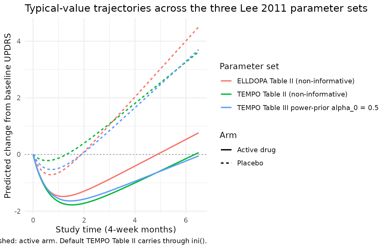

The three sets agree on the qualitative picture (placebo arm progresses; active arm dips and stays near baseline) but quantitatively differ. ELLDOPA has a steeper placebo slope (0.99 vs 0.73 UPDRS/month) and a stronger placebo symptomatic dip (1.93 vs 1.12 UPDRS), reflecting the paper’s observation that “both placebo ( $\beta_0$ ) and drug effects ( $\beta_1$ ) on slope show the same direction” across the two trials but differ in magnitude. The power-prior fit sits between the two non-informative-prior fits as expected.

Assumptions and deviations (Errata)

Source-paper time-unit typo. Lee 2011 Table II column headers state Delta UPDRS score/week for the slope-domain parameters and Delta UPDRS/week for the symptomatic-effect parameters. The math reproducing the paper’s own published placebo prediction (3.62 at week 26) demonstrates that the parameters are actually per 4-week month rather than per week: $0.73 \cdot 26 - 1.12 \cdot (1 - e^{-1.46 \cdot 26}) = 17.86$ vs. published 3.62 if interpreted as /week; vs. $0.73 \cdot 6.5 - 1.12 \cdot (1 - e^{-1.46 \cdot 6.5}) = 3.625$ if interpreted as /month (4-week months). The ELLDOPA placebo slope of 0.99 per week would imply roughly 50 UPDRS units of progression per year, well above the literature value of about 10-12 per year for early Parkinson’s disease, providing a second independent confirmation. Additionally the $\gamma$ “/week” header is dimensionally suspect because symeff appears multiplied by the unitless $1 - e^{-k_{e0} t}$ in equation 1. The model file therefore documents the parameters as UPDRS/month and UPDRS, and the time axis used throughout this vignette is 4-week months. A downstream user wanting to fit the model with time in weeks should multiply beta0, beta1, and lke0 by an appropriate weeks-per-month conversion factor.
Sigma matrix sign-of-life check. The source paper’s printed covariance matrix $\Sigma$ on page 510 shows the variances in the off-diagonal positions and zeros on the diagonal. This is inconsistent with the Methods text statement that “ $b_{1i}$ and $b_{2i}$ were assumed to be independent” – under independence the off-diagonals would be zero and the diagonals would carry the variances. The model file assumes the printed $\Sigma$ is a transcription error (the on-diagonal independence reading) and uses etaslope ~ 0.47 and etasymeff ~ 18.61 from the paper’s w^2_1 and w^2_2 Table II columns. A reader concerned about the off-diagonal printing should consult the published paper directly; the encoded model matches the verbal description.
Drug effect represented as a binary indicator, not via PK exposure. The model has no depot / central compartment and no exposure response. The active-arm shift on $\beta_0$ and $\gamma_0$ is the entire pharmacology of the model – it captures the within-trial active-vs-placebo contrast, not the rasagiline dose-response or the carbidopa-levodopa dose-response that would be needed to extrapolate to new dose levels. The Lee 2011 paper notes that the two rasagiline dose levels (1 and 2 mg/day) in TEMPO had overlapping disease-progression time profiles and were therefore pooled into a single active arm. To use this model for a future rasagiline trial at a novel dose, an exposure response would need to be added; the model as published only supports rasagiline-pooled vs placebo and carbidopa-levodopa-pooled vs placebo contrasts.
Default ini() values are the TEMPO non-informative-prior Table II posterior means. The validation above also documents the ELLDOPA Table II fit and the TEMPO Table III power-prior fit at $\alpha_0 = 0.5$ . Alternative defaults can be loaded by deriving from this model via ini(mod) <- .... The paper’s main quantitative argument – that borrowing strength from ELLDOPA reduces the posterior uncertainty on the TEMPO parameters – is visible directly in the Table III standard deviations (e.g., for $\beta_1$ , SD shrinks from 0.11 with $\alpha_0 = 0$ to 0.06 with $\alpha_0 = 1.0$ ). The current model file’s ini() does not encode posterior SDs directly; downstream Bayesian uses of this model can specify priors externally.
Population metadata partially imputed. Lee 2011 is a methodology paper and does not retabulate the TEMPO or ELLDOPA baseline demographic tables; it states only that “mean ages were 61 and 64 years for ELLDOPA and TEMPO studies, most patients (more than 90%) were Caucasian, and more male patients were enrolled than female patients in both studies.” Exact subject counts, per-arm enrollment numbers, sex percentages, age ranges, and weight distributions are recorded as NA_* in population. A future revision drawing on the original TEMPO and ELLDOPA trial reports could fill these in.
paper_specific_etas declaration. The eta names etaslope and etasymeff deviate from the canonical pairing eta + l<parameter> (which would imply log-transformed primary parameters lslope / lsymeff). The source paper, however, places the random effects directly on linear-scale slope_i and symeff_i, and the primary parameters beta0 / beta1 / gamma0 / gamma1 are signed linear-scale fixed effects rather than log-transformed positive parameters. The model file therefore declares paper_specific_etas <- c("etaslope", "etasymeff") so checkModelConventions() accepts the names. The convention check passes (lint-conventions.R exit 0); see the SKILL.md “Paper-specific etas” reference for the broader pattern.
No PKNCA validation. Standard popPK validation against PKNCA Cmax / AUC / half-life does not apply to a disease-progression model with no exposure compartment. The validation here is instead by direct algebraic reproduction of the paper’s published 3.62 placebo prediction at week 26, plus stochastic-VPC-style envelopes for the typical-value population. This follows the disease-progression / endogenous-model validation pattern documented in the SKILL.md endogenous-validation.md reference.
Trial-design extensions documented in the paper but not encoded in this model. Lee 2011 also describes a dropout sub-model (MAR mechanism with $P(R_{it} = 1) = \text{logit}^{-1}(\delta_0 + \delta_1 \cdot Y_{it-1})$ ) for trial-simulation purposes, with parameters fitted to give roughly 20% dropout at 20-24 weeks, 13% at 16 weeks, and 10% at 12 weeks. The dropout parameters $\delta_0$ and $\delta_1$ are described as “manipulated depending on the study duration” but specific values are not tabulated. The model file does not include the dropout sub-model; downstream trial-simulation use cases that need it should add it as an extension.