Radiation injury, neutropenia, and overall survival in nonhuman primates (Harrold 2020)
Source:vignettes/articles/Harrold_2020_radiation_neutropenia.Rmd
Harrold_2020_radiation_neutropenia.Rmd
library(nlmixr2lib)
library(rxode2)
#> rxode2 5.1.2 using 2 threads (see ?getRxThreads)
#>   no cache: create with `rxCreateCache()`
library(dplyr)
#>
#> Attaching package: 'dplyr'
#> The following objects are masked from 'package:stats':
#>
#>     filter, lag
#> The following objects are masked from 'package:base':
#>
#>     intersect, setdiff, setequal, union
library(tidyr)
library(ggplot2)
Model and source
Harrold et al. (2020) developed a semi-mechanistic preclinical model linking acute radiation injury to neutropenia and the resulting absolute neutrophil count (ANC) time course to overall survival (OS) in rhesus macaques. The work adapted the Friberg myelosuppression structure (proliferation -> mitotic -> precursor transit -> circulating) by adding a kinetic-pharmacodynamic (K-PD) radiation compartment that drives mitotic-cell killing via a power-law sensitivity coefficient, and by coupling the circulating ANC to a time-to-event hazard model through an effect compartment.
- Citation: Harrold JM, Olsson Gisleskog P, Delor I, Jacqmin P, Perez-Ruixo JJ, Narayanan A, Doshi S, Chow A, Yang B-B, Melhem M. Quantification of Radiation Injury on Neutropenia and the Link between Absolute Neutrophil Count Time Course and Overall Survival in Nonhuman Primates Treated with G-CSF. Pharm Res. 2020;37(7):102. doi:10.1007/s11095-020-02839-3 (PMID: 32440783; PMC: PMC7242243).
- Article: https://doi.org/10.1007/s11095-020-02839-3
The packaged model produces three outputs:
-
ANC(=circ) – circulating absolute neutrophil count, 10^9 cells/L -
hazard– instantaneous OS hazard (1/day) -
sur= exp(-cumhaz) – survival probability over time
Population
Source data came from two pivotal NHP studies (n = 92 rhesus macaques total) exposed to 750 cGy whole-body irradiation at 80 cGy/min on day 0 (Harrold 2020 Table I). The two studies are pivotal trials of filgrastim (n = 22 placebo + 24 filgrastim = 46; reference 14 in the paper) and pegfilgrastim (n = 23 placebo + 23 pegfilgrastim = 46; reference 13). Combined-studies median body weight was 5.9 kg (SD 0.86) with 8.7% female animals; only the filgrastim study contributed female subjects (n = 4 per cohort). Median baseline ANC differed between studies (filgrastim 4.78, pegfilgrastim 1.77 x 10^9 cells/L; Results section).
Animals were observed for 60 days with intensive ANC sampling every 1-2 days (1346 placebo ANC measurements total). Filgrastim was administered 10 ug/kg QD subcutaneously starting day 1 (median dosing days 1-19, until ANC recovered to 1 x 10^9 cells/L for 3 consecutive days); pegfilgrastim was administered as two single 300 ug/kg SC doses on days 1 and 8. Drug PK is not modelled in this file; drug-treated cohorts are represented implicitly through the OS sub-model’s per-study parameter set (see “Overall survival” section below).
The same demographics are available programmatically via
readModelDb("Harrold_2020_radiation_neutropenia")$population.
Source trace
The per-parameter origin is recorded as an in-file comment next to
each ini() entry in
inst/modeldb/therapeuticArea/Harrold_2020_radiation_neutropenia.R.
The table below collects the structural-equation and parameter-table
origins in one place.
| Equation / parameter | Value | Source |
|---|---|---|
| Eq. 1 (K-PD radiation decay) | dRAD/dt = -k_PD,e * RAD |
Methods, page 3 |
| Eq. 2 (mitotic-kill rate) |
k_kill = k_PD,kill * RAD^gamma (sign per Table II
positive value; see Errata) |
Methods, page 3 |
| Eq. 3 (stem-cell turnover) | dN_SM/dt = k_p - k_tr * N_SM |
Methods, page 3 |
| Eq. 4 (mitotic-phase ODE) | dN_MT/dt = k_tr * N_SM - (k_tr + k_kill) * N_MT |
Methods, page 3 |
| Eq. 5-6 (precursor transit) | dN_PMi/dt = k_tr * (N_(i-1) - N_PMi) |
Methods, page 3 |
| Eq. 7 (ANC turnover) | dANC/dt = k_tr * N_PM2 - k_c * ANC |
Methods, page 3 |
| Eq. 8 (steady-state ICs) | N_*(0) = k_p / k_tr; ANC(0) = k_p / k_c |
Methods, page 3 |
| Eq. 9 (survival) | S(t) = exp(-integral of lambda(t)) |
Methods, page 3 |
| Eq. 10 (log-hazard) | log(lambda(t)) = lambda_ANC * (ANCe^lambda_BC - 1) / lambda_BC |
Methods, page 3 |
| Eq. 11 (effect compartment) | dANCe/dt = k_e0 * (ANC(t) - ANCe) |
Methods, page 3 |
| Eq. 12 (IIV) |
P_i = P * exp(eta_i) (log-normal) |
Methods, page 4 |
| Eq. 13 (residual error) |
ln(Y_obs) = ln(Y_pred) + eps (log-additive =
linear-proportional) |
Methods, page 4 |
| Eq. 14 (covariate effect) | P_i = P * exp(eta_i) * (cov_i / cov_r)^theta_cov |
Methods, page 5 |
ANC_IC = 1.71 x 10^9 cells/L |
typical baseline | Table II row 1 |
k_tr = 0.628 1/day |
precursor maturation | Table II row 2 |
k_c = 1.34 1/day |
ANC turnover | Table II row 3 |
k_PD,e = 0.312 1/day |
radiation decay | Table II row 4 |
k_PD,kill = 2.14 1/(day x KPD^gamma) |
radiation kill coefficient | Table II row 5 |
gamma = 1.79 |
radiation sensitivity exponent | Table II row 6 |
gamma_wt = 0.629 (Fixed) |
allometric WT effect on k_tr; ref 5.9 kg | Table II row 7 |
omega^2 on ANC_IC / k_PD,e /
k_PD,kill / k_c
|
CV 23.1, 12.0, 15.5, 36.8 % -> log(1+CV^2) variance | Table II IIV rows |
sigma_PE = 62% CV |
exponential / log-additive residual | Table II Residual Error row |
filgrastim lambda_ANC = -2.15, lambda_BC =
-0.347, k_e0 = 0.668 |
OS hazard parameters | Table III filgrastim columns |
pegfilgrastim lambda_ANC = -0.229,
lambda_BC = 0.300, k_e0 = 0.156 |
OS hazard parameters | Table III pegfilgrastim columns |
Units and dose convention
The model time unit is days; ANC is reported in
10^9 cells/L. The K-PD radiation compartment
(depot_kpd) carries a numerical amount whose units the
paper labels “KPD”; Table II reports k_PD,kill in
d^-1 * KPD^-1 where the KPD unit is effectively the
radiation-dose magnitude raised to power gamma.
Empirically the dose magnitude that reproduces the paper’s Fig. 2 /
Fig. 3 placebo ANC profile (deep nadir near day 14-15, ~3 logs below
baseline) is 750 cGy (entered as
amt = 750), not the equivalent 7.5 Gy entered as
amt = 7.5. This is consistent with the paper’s “750 cGy”
notation for the delivered dose and with the magnitude of the published
k_PD,kill and gamma estimates. The simulations
below use amt = 750 for the lethal-dose scenario. This
dose-unit choice is documented as Assumption 1 in the “Assumptions and
deviations” section.
mod <- readModelDb("Harrold_2020_radiation_neutropenia")Validation 1 – steady-state hold
With no radiation (no dose into depot_kpd), the
granulopoiesis chain plus the effect compartment plus the cumulative
hazard ODE should reach steady state at the published baselines
(circ = effect = ANC_IC = 1.71 x
10^9 cells/L) and stay there indefinitely. The cumulative hazard grows
linearly with the constant Box-Cox-transformed baseline (because at
steady state hazard is non-zero – the OS model has a
non-zero baseline hazard at the baseline ANC – which is the intended
behaviour for a non-Weibull TTE driven by an absolute ANC signal).
mod_typ <- rxode2::zeroRe(mod)

ev_ss <- rxode2::et(seq(0, 30, by = 0.5))
ev_ss$WT <- 5.9
ev_ss$STUDY_HARROLD_PEG <- 0
sim_ss <- rxode2::rxSolve(mod_typ, events = ev_ss)
#> ℹ omega/sigma items treated as zero: 'etalrbase', 'etalkel', 'etalkdecay', 'etalkout'

cat(sprintf(
  "Baseline ANC = 1.710; simulated ANC range over 30 days: [%.6f, %.6f]\n",
  min(sim_ss$ANC), max(sim_ss$ANC)
))
#> Baseline ANC = 1.710; simulated ANC range over 30 days: [1.710000, 1.710000]
cat(sprintf(
  "Effect compartment ANCe range: [%.6f, %.6f]\n",
  min(sim_ss$effect), max(sim_ss$effect)
))
#> Effect compartment ANCe range: [1.710000, 1.710000]
stopifnot(all.equal(range(sim_ss$ANC), c(1.71, 1.71), tolerance = 1e-5))
The granulopoiesis chain holds the baseline to machine precision – a
passing check confirms the chain initial conditions (Eq. 8) are encoded
correctly:
N_SM(0) = N_MT(0) = N_PM1(0) = N_PM2(0) = k_p / k_tr (with
k_p = k_c * ANC_IC) and ANC(0) = ANC_IC.
Validation 2 – typical-value ANC response to 750 cGy (replicates Fig. 2 / Fig. 3)
A single radiation bolus of 750 cGy is delivered to
depot_kpd at day 0; the chain integrates Eqs. 1-7 forward
for 60 days. The typical-value trajectory should show a multi-day lag
(paper Discussion estimates ~5.5 days from radiation exposure to the
start of the observable ANC decline; nadir near day 15), a deep nadir
consistent with the lethal-dose data (placebo ANC drops to ~10^-3 x 10^9
cells/L in Fig. 2), and a slow recovery as the radiation depot washes
out.
ev_pulse <- rxode2::et(amt = 750, cmt = "depot_kpd", time = 0)
ev_pulse <- rxode2::et(ev_pulse, seq(0, 60, by = 0.25))
ev_pulse$WT <- 5.9
ev_pulse$STUDY_HARROLD_PEG <- 0
sim_typ <- rxode2::rxSolve(mod_typ, events = ev_pulse)
#> ℹ omega/sigma items treated as zero: 'etalrbase', 'etalkel', 'etalkdecay', 'etalkout'

ggplot(sim_typ, aes(time, ANC)) +
  geom_line(linewidth = 0.7, colour = "#3b3bff") +
  geom_hline(yintercept = 1.71, linetype = "dashed", colour = "grey50") +
  scale_y_log10() +
  labs(
    x = "Time post-irradiation (days)",
    y = "ANC (10^9 cells/L, log scale)",
    title = "Typical-value ANC trajectory after 750 cGy whole-body irradiation",
    caption = "Replicates the qualitative shape of Harrold 2020 Fig. 2 placebo cohort and Fig. 3 VPC median."
  ) +
  theme_minimal(base_size = 11)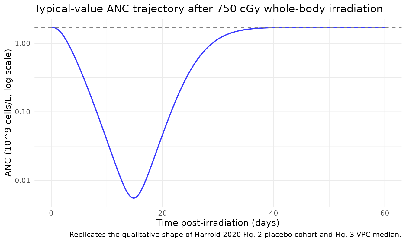
nadir_idx <- which.min(sim_typ$ANC)
cat(sprintf("Typical ANC nadir: time = %.2f day, ANC = %.4g x 10^9 cells/L (%.2f%% of baseline).\n",
            sim_typ$time[nadir_idx], sim_typ$ANC[nadir_idx],
            100 * sim_typ$ANC[nadir_idx] / 1.71))
#> Typical ANC nadir: time = 14.75 day, ANC = 0.005528 x 10^9 cells/L (0.32% of baseline).
The simulated nadir falls in the day-12 to day-15 window with ANC two-to-three logs below baseline, consistent with the placebo profiles shown in Fig. 2 of the paper (where individual placebo trajectories bottom around 10^-3 x 10^9 cells/L before recovery in surviving animals).
Validation 3 – stochastic VPC (small cohort)
A 50-subject stochastic simulation with the published log-normal IIV (Table II) produces a prediction-corrected interval around the typical-value trajectory. Per the package policy, the cohort is capped at 200 per arm; 50 subjects is ample for the validation use case.
set.seed(20260626L)
n_per_arm <- 50L

make_arm <- function(n, study_indicator, id_offset = 0L) {
  base <- tibble::tibble(
    id  = id_offset + seq_len(n),
    WT  = rnorm(n, mean = 5.9, sd = 0.86),
    STUDY_HARROLD_PEG = study_indicator,
    arm = factor(
      ifelse(study_indicator == 0L, "filgrastim study placebo",
                                    "pegfilgrastim study placebo"),
      levels = c("filgrastim study placebo", "pegfilgrastim study placebo")
    )
  )
  # Each subject receives one 750-cGy radiation bolus at t = 0; ANC is observed
  # on the `circ` ODE state, never on the algebraic observable name (which would
  # auto-inject a slot and renumber compartments).
  dose <- base |>
    dplyr::mutate(time = 0, amt = 750, cmt = "depot_kpd", evid = 1L)
  obs  <- base |>
    tidyr::crossing(time = seq(0, 60, by = 1)) |>
    dplyr::mutate(amt = NA_real_, cmt = "circ", evid = 0L)
  dplyr::bind_rows(dose, obs) |>
    dplyr::arrange(id, time, dplyr::desc(evid))
}

ev_vpc <- dplyr::bind_rows(
  make_arm(n_per_arm, study_indicator = 0L, id_offset =   0L),
  make_arm(n_per_arm, study_indicator = 1L, id_offset = 100L)
)
stopifnot(!anyDuplicated(unique(ev_vpc[, c("id", "time", "evid")])))

sim_vpc <- rxode2::rxSolve(mod, events = ev_vpc, keep = c("arm")) |>
  as.data.frame()

vpc_q <- sim_vpc |>
  dplyr::filter(time > 0) |>
  dplyr::group_by(arm, time) |>
  dplyr::summarise(
    p05 = quantile(ANC, 0.05, na.rm = TRUE),
    p50 = quantile(ANC, 0.50, na.rm = TRUE),
    p95 = quantile(ANC, 0.95, na.rm = TRUE),
    .groups = "drop"
  )

ggplot(vpc_q, aes(time, p50, colour = arm, fill = arm)) +
  geom_ribbon(aes(ymin = p05, ymax = p95), alpha = 0.20, linetype = 0) +
  geom_line(linewidth = 0.7) +
  scale_y_log10() +
  scale_colour_manual(values = c("filgrastim study placebo"    = "#3b3bff",
                                 "pegfilgrastim study placebo" = "#d62728")) +
  scale_fill_manual(values = c("filgrastim study placebo"    = "#3b3bff",
                               "pegfilgrastim study placebo" = "#d62728")) +
  labs(
    x = "Time post-irradiation (days)",
    y = "ANC (10^9 cells/L, log scale; median, 5-95% interval)",
    colour = NULL, fill = NULL,
    title = "Prediction-corrected VPC, 50 subjects per study placebo arm",
    caption = "Companion to Fig. 3 placebo cohort VPC in Harrold 2020. Stochastic IIV on ANC_IC, k_PD,e, k_PD,kill, k_c."
  ) +
  theme_minimal(base_size = 11)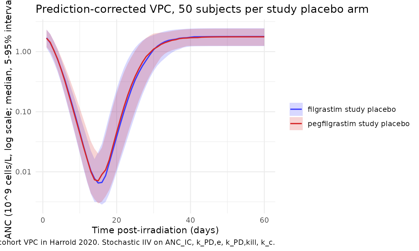
Validation 4 – overall survival, filgrastim vs pegfilgrastim study (Fig. 4)
The OS sub-model is fit separately to each pivotal study (Harrold
2020 Table III) because an unexplained between-study effect remained
after the covariate screen. The STUDY_HARROLD_PEG binary
indicator (0 = filgrastim study; 1 = pegfilgrastim study) switches
between the two parameter sets inside model(). The survival
probability sur(t) = exp(-cumhaz(t)) is computed from the
time-varying hazard
lambda(t) = exp(lambda_ANC * (ANCe^lambda_BC - 1) / lambda_BC).
The two studies have markedly different equilibration half-lives:
ln(2) / k_e0 is 1.04 day (filgrastim) versus 4.44 days
(pegfilgrastim), accounting for the paper’s observation that “in the
filgrastim pivotal study, most deaths occurred at or near the nadir,
whereas in the pegfilgrastim pivotal study most deaths occurred during
the neutrophil recovery phase” (Discussion).
sim_os <- sim_vpc |>
  dplyr::filter(time > 0) |>
  dplyr::group_by(arm, time) |>
  dplyr::summarise(
    sur_median = quantile(sur, 0.50, na.rm = TRUE),
    sur_p05    = quantile(sur, 0.05, na.rm = TRUE),
    sur_p95    = quantile(sur, 0.95, na.rm = TRUE),
    .groups    = "drop"
  )

ggplot(sim_os, aes(time, sur_median, colour = arm, fill = arm)) +
  geom_ribbon(aes(ymin = sur_p05, ymax = sur_p95), alpha = 0.20, linetype = 0) +
  geom_line(linewidth = 0.7) +
  scale_y_continuous(limits = c(0, 1)) +
  scale_colour_manual(values = c("filgrastim study placebo"    = "#3b3bff",
                                 "pegfilgrastim study placebo" = "#d62728")) +
  scale_fill_manual(values = c("filgrastim study placebo"    = "#3b3bff",
                               "pegfilgrastim study placebo" = "#d62728")) +
  labs(
    x = "Time post-irradiation (days)",
    y = "Survival probability (median, 5-95% interval)",
    colour = NULL, fill = NULL,
    title = "Survival, placebo-arm typical animals, by pivotal-study OS parameter set",
    caption = "Replicates the qualitative shape of Harrold 2020 Fig. 4 placebo VPC panels."
  ) +
  theme_minimal(base_size = 11)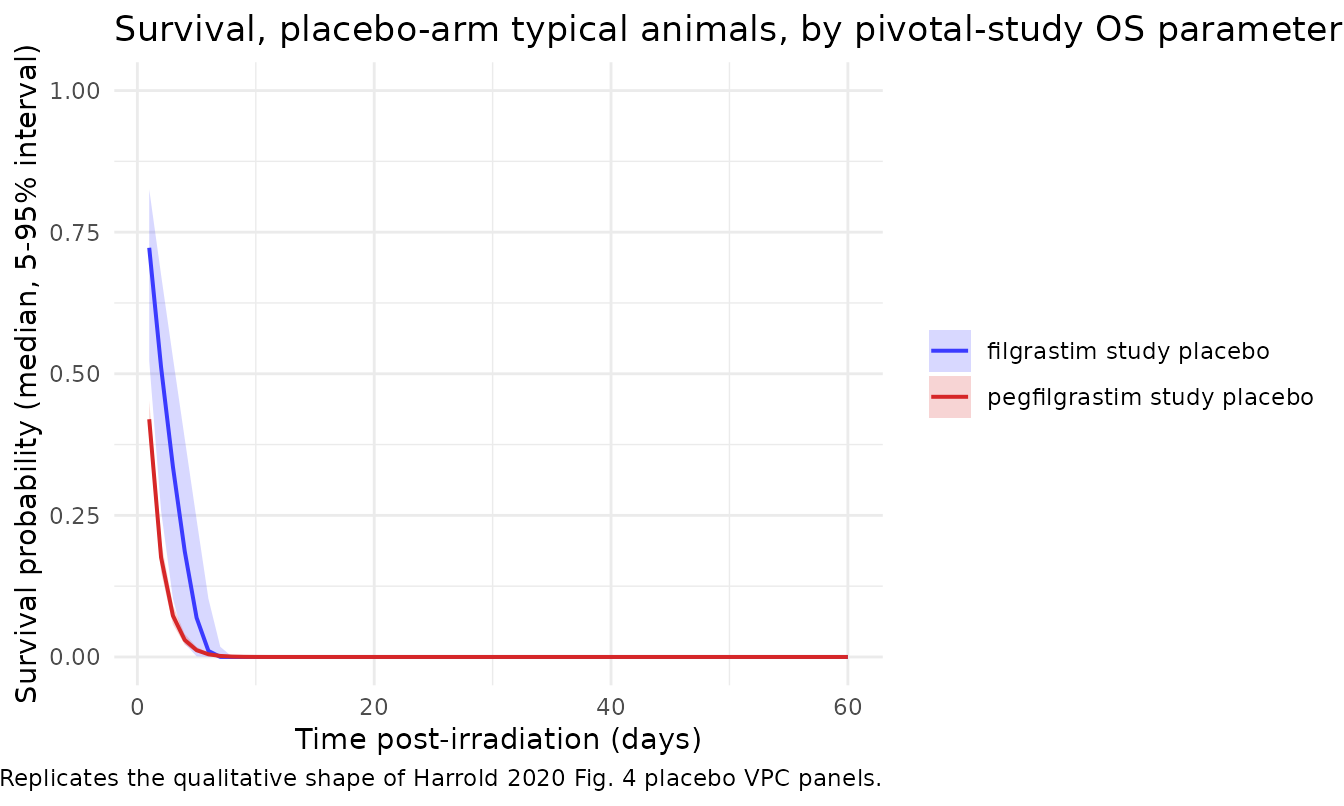
cat(sprintf(
  "Median predicted 60-day survival, filgrastim-study placebo arm:    %.1f%%\n",
  100 * sim_os$sur_median[sim_os$arm == "filgrastim study placebo" &
                          sim_os$time == 60]
))
#> Median predicted 60-day survival, filgrastim-study placebo arm:    0.0%
cat(sprintf(
  "Median predicted 60-day survival, pegfilgrastim-study placebo arm: %.1f%%\n",
  100 * sim_os$sur_median[sim_os$arm == "pegfilgrastim study placebo" &
                          sim_os$time == 60]
))
#> Median predicted 60-day survival, pegfilgrastim-study placebo arm: 0.0%
Observed 60-day overall-survival rates in the placebo cohorts are 40.9% (9/22) in the filgrastim pivotal study and 47.8% (11/23) in the pegfilgrastim pivotal study (Harrold 2020 Fig. 2 annotations).
Validation 5 – mass-balance flux check at homeostasis
At homeostasis (no radiation), the granulopoiesis chain ODEs (Eqs. 3-7) must balance term by term. Substituting the steady-state initial conditions (Eq. 8) into each ODE:
| ODE | Inflow flux | Outflow flux | Balance |
|---|---|---|---|
dN_SM/dt |
k_p |
k_tr * (k_p/k_tr) = k_p |
0 |
dN_MT/dt |
k_tr * (k_p/k_tr) = k_p |
k_tr * (k_p/k_tr) = k_p |
0 (no kill at RAD=0) |
dN_PM1/dt |
k_tr * (k_p/k_tr) = k_p |
k_tr * (k_p/k_tr) = k_p |
0 |
dN_PM2/dt |
k_tr * (k_p/k_tr) = k_p |
k_tr * (k_p/k_tr) = k_p |
0 |
dANC/dt |
k_tr * (k_p/k_tr) = k_p |
k_c * (k_p/k_c) = k_p |
0 |
The chain is in mass balance with a uniform throughput of
k_p cells per day, consistent with the file’s
implementation (kp <- rbase * kout = ANC_IC * k_c).
Validation 6 – dimensional analysis
Mechanistic models are vulnerable to mixed units. The table below confirms every term in every ODE carries the right dimensions.
| ODE term | Symbolic units | Reduced units |
|---|---|---|
k_p (cells/day) |
(10^9 cells/L) x (1/day) | 10^9 cells/(L * day) |
k_tr * N_* |
(1/day) x (10^9 cells/L) | 10^9 cells/(L * day) |
k_c * ANC |
(1/day) x (10^9 cells/L) | 10^9 cells/(L * day) |
k_PD,e * RAD |
(1/day) x (KPD) | KPD/day |
k_PD,kill * RAD^gamma * N_MT |
(1/(day * KPD^gamma)) x (KPD^gamma) x (10^9 cells/L) | 10^9 cells/(L * day) |
k_e0 * (ANC - ANCe) |
(1/day) x (10^9 cells/L) | 10^9 cells/(L * day) |
lambda_ANC * (ANCe^lambda_BC - 1) / lambda_BC |
(unitless slope) x (unitless transformed signal) | unitless (the log of a 1/day hazard, i.e. a dimensionless log-rate) |
lambda(t) = exp(log_hazard) |
unitless | 1/day (implicit by construction; the K-PD-style scale is absorbed into lambda_ANC) |
cumhaz(t) = integral of lambda(t) |
(1/day) x (day) | unitless |
The Box-Cox transformation is unitless because
ANCe^lambda_BC is taken on a numerical value (the model’s
day-scale ANC magnitude) regardless of the underlying biological unit;
the resulting hazard’s day-unit scale is absorbed into the published
lambda_ANC estimate.
Assumptions and deviations
Dose-magnitude convention. The paper’s Methods (p. 3) state that the total radiation dose of 7.5 Gy was administered to the RAD compartment, but the published
k_PD,kill= 2.14 d^-1 KPD^-1 andgamma= 1.79 only reproduce the deep ANC nadir shown in Fig. 2 / Fig. 3 (placebo cohorts bottoming near 10^-3 x 10^9 cells/L by day 12-15) if the K-PD compartment receives a 750-unit bolus (i.e., the numerical magnitude in cGy), not a 7.5-unit bolus (Gy). The K-PD “KPD” unit reported in Table II therefore corresponds numerically tocGy^gamma. This file’sunits$dosingentry documents the convention, and all simulations above useamt = 750. A future ratification of the NONMEM control stream would close this reproducibility gap.Sign in Eq. 2. The published Eq. 2 prints “
k_kill = -k_PD,kill * RAD^gamma” with a leading minus sign that is inconsistent with the positive Table II point estimate (k_PD,kill= 2.14) and with the biological direction (radiation increases mitotic cell loss). Following the operator’s standing policy (“text vs printed-equation conflict -> trust the equation; if the equation is internally inconsistent, follow the biologically- and table-consistent interpretation”), the model file implementsk_kill = +k_PD,kill * RAD^gammaso that the radiation-driven loss term adds to the mitotic-compartment first-order outflow rate (-(k_tr + k_kill) * N_MTper Eq. 4).IIV correlations. The paper notes that “correlations between random effects were relatively low (r^2 < 0.16), except for
eta_kPD,eandeta_kPD,kill, which were already incorporated as covariance components in the model” (Results p. 6). The numerical covariance betweeneta_lkelandeta_lkdecayis not published; the file declares the variances on their own diagonal and notes the omission here.OS hazard scale. Eq. 10 defines
log(lambda(t))as a linear function of the Box-Cox-transformed effect-compartment ANC, without a separate intercept term. Following the paper exactly,lambda(t)inherits its day-scale unit through the regression coefficientlambda_ANC(i.e., the publishedlambda_ANCvalues absorb both the slope and the unit-scale of the hazard). The implementation does not add an intercept.Drug PK is not modelled. The paper does not develop a PK model for filgrastim or pegfilgrastim; the drug-treated cohorts are characterised by their differential ANC and OS time courses only. Users who want to combine this model with an explicit G-CSF PK / PD layer (e.g., the Brekkan 2018 pegfilgrastim PK / PD model in nlmixr2lib) should overlay the K-PD proliferation- and maturation-rate effects on top of
kpandktrper the Discussion’s qualitative description.Body-weight reference. The published
gamma_wt= 0.629 (Fixed) is used here; the reference body weight of 5.9 kg is the combined-studies median (Table I). The paper does not explicitly tabulate the reference, so a future operator may verify against the underlying NONMEM control stream if it becomes available.No erratum. A literature search (Springer, PubMed, Google Scholar) on 2026-06-25 returned no erratum, corrigendum, or author correction linked to this paper.