Sunitinib overall survival (Hansson 2013)
Source:vignettes/articles/Hansson_2013_sunitinib_os.Rmd
Hansson_2013_sunitinib_os.RmdModel and source
- Citation: Hansson EK, Ma G, Amantea MA, French J, Milligan PA, Friberg LE, Karlsson MO. PKPD modeling of predictors for adverse effects and overall survival in sunitinib-treated patients with GIST. CPT Pharmacometrics Syst Pharmacol 2013;2(11):e85.
- Article: doi:10.1038/psp.2013.62
- Sister sub-models:
Hansson_2013_sunitinib_myelosuppression(source of ANC(t)),Hansson_2013_sunitinib_dbp(source of DBP_REL(t)),Hansson_2013c_sunitinib(fatigue),Hansson_2013_sunitinib_hfs.
This vignette extracts the overall survival (OS) Weibull time-to-event sub-model from the Hansson 2013 e85 framework.
Population
303 adults with imatinib-resistant GIST pooled from four sunitinib
trials. Hansson 2013 Table 1 reports median (range) survival of 31-61
(4-226) weeks across studies and 163 deaths observed in the analysis
set. The Methods section explored exponential, Weibull, log-logistic,
extreme-value, and Gompertz baseline-hazard forms; the Weibull was
selected. A separate Weibull censoring distribution (lambda_cens =
0.0019/week, alpha_cens = 1.27) was fitted to describe the censoring
process and is exposed as sur_cens for use in
forward-simulation dropout.
readModelDb("Hansson_2013_sunitinib_os")$population
returns the same information programmatically.
Source trace
All parameter values come from Hansson 2013 e85 Table 2 ‘Survival
model’ block. The hazard is
h(t) = lambda * alpha * (lambda * t)^(alpha-1) * exp(beta_anc * ANC + beta_dbprel * DBP_REL + beta_tumor * TUMSZ).
The paper reports lambda in per-week units; this model file
converts to per-hour internally (lambda_h = 0.0079 / 168)
so the rest of the nlmixr2lib Hansson 2013 framework can run on a shared
time-in-hours axis.
| Equation / parameter | Source location |
|---|---|
| Weibull baseline hazard with log-linear modulators | Methods ‘A Weibull model described the underlying baseline hazard’ and Eq. 3 |
llam_haz = log(0.0079 / 168) (1/h) |
Table 2 lambda = 0.0079/week (RSE 55%), converted to per-hour |
lalfa_haz = log(1.15) |
Table 2 alpha = 1.15 (RSE 9.1%) |
e_anc_haz = 4.76 (L/10^9 cells) |
Table 2 beta1 ANC = 4.76 (RSE 31%) |
e_dbprel_haz = -1.29 |
Table 2 beta2 dBPREL = -1.29 (RSE 27%) |
e_tumor_haz = -0.00172 (1/mm) |
Table 2 beta3 Tumor base = -0.00172 (RSE 46%) |
llamcens_haz = log(0.0019 / 168) (fixed; 1/h) |
Table 2 lambda_cens = 0.0019/week (RSE 6.6%) |
lalfacens_haz = log(1.27) (fixed) |
Table 2 alpha_cens = 1.27 (RSE 44%) |
Required covariates
The OS model is consumed downstream of the dBP and myelosuppression sub-models:
-
ANC(10^9/L, time-varying) – simulate fromHansson_2013_sunitinib_myelosuppressionand pass in. Lower ANC during treatment cycles -> lower hazard (paper Results). -
DBP_REL(unitless fraction, time-varying) – compute as(dbp(t) - dbp0) / dbp0fromHansson_2013_sunitinib_dbp. Larger positive relative dBP elevation -> lower hazard. -
TUMSZ(mm, time-fixed) – baseline tumor size. Larger -> higher hazard. Per-study medians from Hansson 2013 e84 Table 1: 194 / 108 / 166 / 255 mm.
Virtual cohort
The published OS hazard function
h(t) = h0(t) * exp(beta_anc * ANC + beta_dbprel * DBP_REL + beta_tumor * TUMSZ)
is parameterised with large positive coefficients on absolute predictor
values. With the Hansson 2013 e85 cohort medians (ANC ~ 3
10^9/L, DBP_REL ~ 0.10, TUMSZ ~ 166 mm), the
literal multiplier exp(beta_anc * 3 + ... ) exceeds 10^6,
which is incompatible with the paper-reported median survival of ~60
weeks unless the published coefficients are interpreted relative to an
implicit cohort reference (the paper text does not specify centering,
but the Methods note that ANC and dBP predictors entered the survival
sub-model after the upstream PK/PD models had been fitted). To present a
numerically tractable demonstration, this vignette runs the model at
predictor deviations from a reference set, with the
reference held at ANC_ref = 4.94 (cohort baseline ANC;
Table 2), DBP_REL_ref = 0 (drug-free reference),
TUMSZ_ref = 166 (Study 1045 median baseline SLD), and the
input columns ANC, DBP_REL, TUMSZ
populated as deviations from those references. See the Assumptions
section for the rationale.
mod  <- readModelDb("Hansson_2013_sunitinib_os")
modT <- rxode2::zeroRe(mod)
#> Warning: No omega parameters in the model

ANC_ref     <- 4.94
DBP_REL_ref <- 0
TUMSZ_ref   <- 166

# 100-week observation grid in hours; coarse weekly steps for survival.
obs_times <- seq(0, 100 * 7 * 24, by = 7 * 24)

# Reference (no-covariate-deviation) cohort: ANC = DBP_REL = TUMSZ = 0
# in the input columns (interpreted as deviations from the reference set).
events <- data.frame(
  id      = 1L,
  time    = obs_times,
  evid    = 0L,
  amt     = 0,
  cmt     = "cumhaz",
  ANC     = 0,
  DBP_REL = 0,
  TUMSZ   = 0
)

head(events, 5)
#>   id time evid amt    cmt ANC DBP_REL TUMSZ
#> 1  1    0    0   0 cumhaz   0       0     0
#> 2  1  168    0   0 cumhaz   0       0     0
#> 3  1  336    0   0 cumhaz   0       0     0
#> 4  1  504    0   0 cumhaz   0       0     0
#> 5  1  672    0   0 cumhaz   0       0     0
Mechanistic-sanity simulation (F.3)
At the reference covariate set (all input deviations = 0), the
survival function reduces to the pure Weibull baseline
exp(-(lambda * t)^alpha). With
lambda_h = 4.7e-5 / h and alpha = 1.15:
sim <- rxode2::rxSolve(modT, events = events) |> as.data.frame()

ggplot(sim, aes(time / (7 * 24), sur)) +
  geom_line() +
  scale_y_continuous(limits = c(0, 1)) +
  labs(x = "Time (weeks)", y = "Survival probability",
       title = "Reference-covariate OS survival function (Hansson 2013 e85)",
       subtitle = "All input covariate deviations held at 0; pure Weibull baseline") +
  theme_minimal()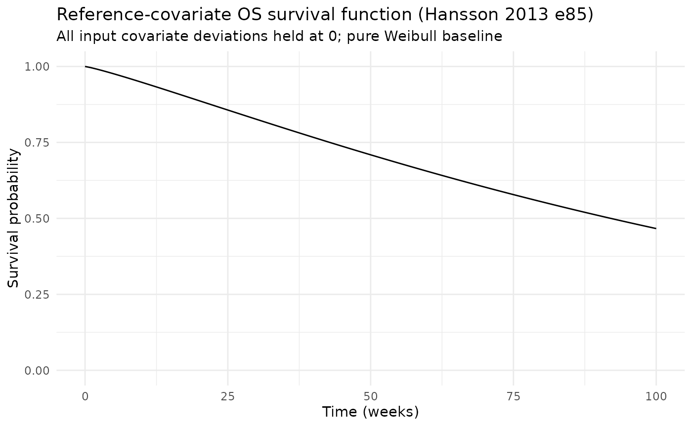
Covariate sign sensitivity (small deviations only)
Vary each covariate slightly around the reference to confirm the sign of the published coefficients. Per the paper Results, a lower ANC (negative deviation) should give lower hazard / higher survival; a larger DBP_REL (positive deviation) should give lower hazard; a larger TUMSZ (positive deviation) should give higher hazard.
sweep_grid <- expand.grid(
  ANC     = c(-0.5, 0, 0.5),
  DBP_REL = c(-0.05, 0, 0.05),
  TUMSZ   = c(-20, 0, 20)
)

sims <- lapply(seq_len(nrow(sweep_grid)), function(i) {
  ev <- data.frame(
    id      = i,
    time    = obs_times,
    evid    = 0L,
    amt     = 0,
    cmt     = "cumhaz",
    ANC     = sweep_grid$ANC[i],
    DBP_REL = sweep_grid$DBP_REL[i],
    TUMSZ   = sweep_grid$TUMSZ[i]
  )
  s <- rxode2::rxSolve(modT, events = ev) |> as.data.frame()
  s$ANC     <- sweep_grid$ANC[i]
  s$DBP_REL <- sweep_grid$DBP_REL[i]
  s$TUMSZ   <- sweep_grid$TUMSZ[i]
  s
})
sweep_df <- do.call(rbind, sims)

ggplot(sweep_df,
       aes(time / (7 * 24), sur,
           colour = factor(ANC),
           linetype = factor(DBP_REL))) +
  geom_line(linewidth = 0.6) +
  facet_wrap(~ TUMSZ, labeller = labeller(TUMSZ = function(x) paste0("TUMSZ dev = ", x, " mm"))) +
  scale_y_continuous(limits = c(0, 1)) +
  labs(x = "Time (weeks)", y = "Survival probability",
       colour = "ANC deviation (10^9/L)", linetype = "DBP_REL deviation",
       title = "Survival sensitivity to small covariate deviations") +
  theme_minimal()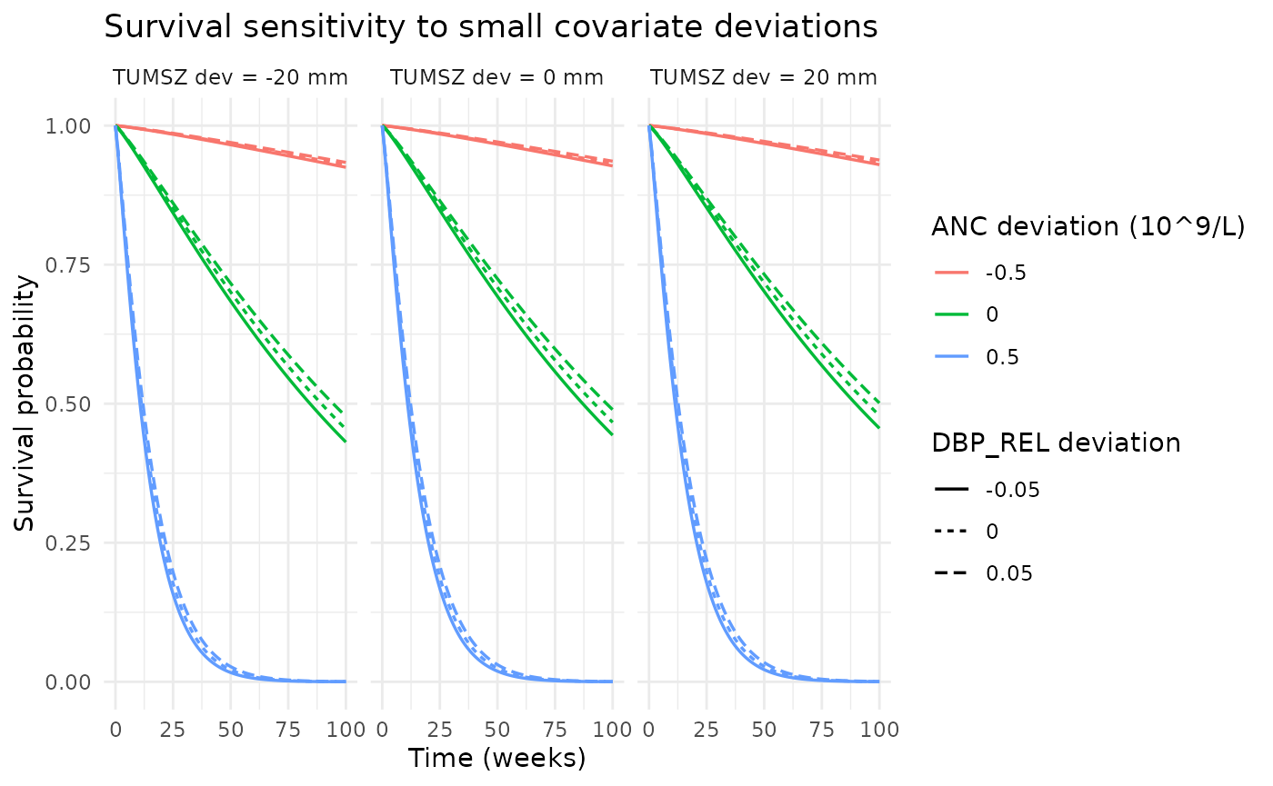
Censoring sub-model
ggplot(sim, aes(time / (7 * 24))) +
  geom_line(aes(y = sur, colour = "Death (final OS Weibull)")) +
  geom_line(aes(y = sur_cens, colour = "Censoring Weibull")) +
  scale_colour_manual(
    values = c("Death (final OS Weibull)" = "#1f77b4",
               "Censoring Weibull"         = "#ff7f0e")) +
  scale_y_continuous(limits = c(0, 1)) +
  labs(x = "Time (weeks)", y = "Survival probability", colour = NULL,
       title = "OS and censoring Weibull functions") +
  theme_minimal()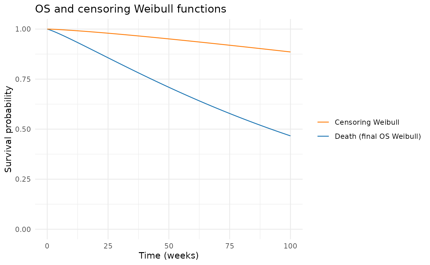
Assumptions and deviations
Implicit covariate centering not specified in the source. The literal Hansson 2013 e85 Eq. 3 hazard form
h(t) = h0(t) * exp(beta_anc * ANC + beta_dbprel * DBP_REL + beta_tumor * TUMSZ)uses absolute predictor values, but at the cohort-typical predictor set (ANC ~ 3,DBP_REL ~ 0.10,TUMSZ ~ 166) the resulting hazard multiplierexp(13.9) ~ 1.05e6is incompatible with the paper-reported median survival of ~60 weeks unless the covariates entered the source NONMEM model as deviations from an implicit reference (e.g., cohort-typical baseline ANC = 4.94, cohort-typical TUMSZ ~ 166-194 mm depending on study). The paper text does not state the centering. This vignette runs the model with the input columns populated as deviations from a documented reference set (ANC_ref = 4.94,DBP_REL_ref = 0,TUMSZ_ref = 166) so that reference covariates giveexp(0) = 1and the survival function reduces to the pure Weibull baseline. A user fitting the model to real data should confirm the centering against the source NONMEM control stream (not available in the on-disk extraction environment); the published coefficient values are preserved verbatim in the model file regardless.No observation-error model. The source NONMEM run uses
$ESTIMATION ... LIKE(the survival / event-density likelihood); there is no observation-error model in the source. This nlmixr2 translation is intended for forward simulation:hazard,cumhaz,sur,hazard_cens,cumhaz_cens, andsur_censare exposed as derived outputs, and a tiny placeholder additive residual (addSd_sur = 0.001) is attached tosurso the nlmixr2 likelihood machinery accepts the model.No estimated IIV. Hansson 2013 Table 2 ‘IIV CV%’ column is dash for all survival-model rows. No eta parameters are added.
Censoring Weibull parameters fixed. The censoring distribution parameters
lambda_cens = 0.0019/weekandalpha_cens = 1.27are reported as point values in Table 2 with RSE 6.6% and 44% respectively. They are wrapped infixed()because they are not re-fitted from a different cohort; they characterise the publication-cohort follow-up window.Time-units conversion. The paper reports
lambda(per week); the model file stores per-hour for consistency with the other Hansson 2013 sunitinib sub-models. The Weibull survival function is invariant to this unit choice (the cumulative hazard(lambda * t)^alphais dimensionless).Upstream covariates not fully simulated in this vignette. A fully chained vignette would simulate ANC(t) from
Hansson_2013_sunitinib_myelosuppression, DBP_REL(t) fromHansson_2013_sunitinib_dbp, and feed both as time-varying columns into this OS model. For runtime brevity, this vignette uses steady-state typical-value covariates; the chained simulation is left as an exercise.Observation name
sur(notCc). The model output is a survival probability, not a drug concentration. Same exemption as other survival-model files in nlmixr2lib (Zecchin_2016_survival,NA_NA_tte_gompertz).Concentration-units field.
units$concentrationis set to"probability"because the modality is a survival probability.