Sunitinib myelosuppression (Hansson 2013)
Source:vignettes/articles/Hansson_2013_sunitinib_myelosuppression.Rmd
Hansson_2013_sunitinib_myelosuppression.RmdModel and source
- Citation: Hansson EK, Ma G, Amantea MA, French J, Milligan PA, Friberg LE, Karlsson MO. PKPD modeling of predictors for adverse effects and overall survival in sunitinib-treated patients with GIST. CPT Pharmacometrics Syst Pharmacol 2013;2(11):e85.
- Article: doi:10.1038/psp.2013.62
- Upstream sVEGFR-3 biomarker dynamics:
Hansson_2013a_sunitinib(DDMODEL00000197, doi:10.1038/psp.2013.61). - Friberg myelosuppression backbone: Friberg LE et al. J Clin Oncol 2002;20(24):4713-4721, doi:10.1200/JCO.2002.02.140.
This vignette extracts the myelosuppression
sub-model from the Hansson 2013 e85 framework – one of five linked
sub-models in the paper alongside diastolic blood pressure
(Hansson_2013_sunitinib_dbp), fatigue
(Hansson_2013c_sunitinib; from the DDMORE bundle),
hand-foot syndrome (Hansson_2013_sunitinib_hfs), and
overall survival (Hansson_2013_sunitinib_os).
Population
The Hansson 2013 e85 analysis pooled data from four sunitinib trials
in 303 adults with imatinib-resistant gastrointestinal stromal tumours
(GIST): Demetri 2006 (study 1004; phase III; 202 active + 47 placebo),
George 2009 (study 1047; phase II continuous dosing; n = 13 in this
subset), Shirao 2010 (study 1045; Japanese phase I/II; n = 36), Maki
2005 (study 013; phase I/II; n = 52). Sunitinib doses ranged from 25 to
75 mg PO QD on 4/2, 2/2, 2/1 weeks-on/off, or continuous schedules
(Table 1). The Japanese cohort (Study 1045) had a lower observed ANC
baseline, so the model carries a separate ANC0 for
RACE_JAPANESE = 1 (3.69 vs 4.94 in 10^9/L; Table 2 row
‘ANC0: Study 45’).
readModelDb("Hansson_2013_sunitinib_myelosuppression")$population
returns the same information programmatically.
Source trace
All parameter values come from Hansson 2013 e85 Table 2
‘Myelosuppression model’ block. The model encodes the paper’s
drug-effect descriptor (sVEGFR-3 REL, the relative reduction in sVEGFR-3
from baseline) by simulating the upstream sVEGFR-3 dynamics in-model
from the Hansson 2013a / DDMODEL00000197 indirect-response covariates
(BAS_SVEGFR3, MRT_SVEGFR3, EC50_SVEGFR3), then computing
svegfr3_rel = (BAS_SVEGFR3 - svegfr3) / BAS_SVEGFR3.
| Equation / parameter | Source location |
|---|---|
| Friberg-Karlsson 5-compartment chain (prol + 3 transit + circ) | Hansson 2013 e85 Methods ‘Myelosuppression model’ |
ktr <- 4 / mtt (Friberg n=3 + prol form) |
Methods ‘three transit compartments reflecting cell maturation’ |
edrug <- Emax * svegfr3_rel / (EC50 + svegfr3_rel) |
Methods ‘An Emax function most appropriately characterized the biomarker-ANC relationship’ |
feed <- (anc0 / circ)^gamma |
Methods ‘a feedback function mimicking the effect of endogenous growth factors’ |
auc <- DOSE / CLI and svegfr3
indirect-response turnover |
Methods ‘Total oral plasma clearance … obtained from a population PK model’ + Hansson_2013a structural form |
svegfr3_rel = (BAS_SVEGFR3 - svegfr3) / BAS_SVEGFR3 |
Methods ‘sVEGFR-3 REL … a more pronounced reduction’ |
lanc0 = log(4.94) (10^9/L; non-Japanese) |
Hansson 2013 Table 2 row ‘ANC0’ = 4.94 (RSE 2.8%) |
e_japanese_anc0 = log(3.69 / 4.94) = -0.292 |
Hansson 2013 Table 2 row ‘ANC0: Study 45’ = 3.69 (RSE 6.9%) |
lmtt = log(248) (h) |
Hansson 2013 Table 2 row ‘MTT’ = 248 h (RSE 3.6%) |
lanc_emax = log(0.520) |
Hansson 2013 Table 2 row ‘ANC Emax’ = 0.520 (RSE 9.1%) |
lanc_ec50 = log(0.552) |
Hansson 2013 Table 2 row ‘ANC EC50’ = 0.552 (RSE 17%) |
gamma = 0.362 |
Hansson 2013 Table 2 row ‘gamma’ = 0.362 (RSE 7.4%) |
etalanc0 + etalanc_emax ~ c(0.1633, 0.04707, 0.01678) |
Hansson 2013 Table 2 IIV CV% (ANC0 = 42%, ANC Emax = 13%), Results section: ‘a correlation between ANC0 and Emax of 90%’ |
etalmtt ~ 0.02852 |
Hansson 2013 Table 2 IIV CV% MTT = 17% |
etalanc_ec50 ~ 0.1929 |
Hansson 2013 Table 2 IIV CV% ANC EC50 = 46% |
addSd_anc = 0.406 |
Hansson 2013 Table 2 ‘Residual error’ = 0.406 on the Box-Cox-transformed scale |
Drug-exposure inputs and required covariates
The model has no PK ODE: sunitinib exposure is summarised per-cycle
as auc = DOSE / CLI (mg*h/L) and fed into a simple-Imax
inhibition of sVEGFR-3 Kin. The required data columns are:
-
DOSE(mg) – time-varying daily sunitinib dose. Held at 50 mg during on-cycles of a 4-weeks-on / 2-weeks-off schedule, 0 mg during off-cycles or placebo. -
CLI(L/h) – per-subject sunitinib clearance from the upstream popPK model. Use 32.819 L/h for typical-cohort simulations (matches Hansson_2013a / Hansson_2013c convention). -
BAS_SVEGFR3(pg/mL) – baseline sVEGFR-3 from the upstream Hansson 2013a biomarker model; typical 63 900 pg/mL. -
MRT_SVEGFR3(h) – mean residence time of sVEGFR-3; typical 401 h. -
EC50_SVEGFR3(mgh/L) – EC50 of the sVEGFR-3 drug effect; typical 1.0 mgh/L. -
RACE_JAPANESE(0/1) – 1 for Study 1045 subjects (lower ANC0); 0 otherwise.
Virtual cohort
mod  <- readModelDb("Hansson_2013_sunitinib_myelosuppression")
modT <- rxode2::zeroRe(mod)
#> ℹ parameter labels from comments will be replaced by 'label()'

# DOSE follows the 4-weeks-on / 2-weeks-off sunitinib schedule.
on_off_dose <- function(time_h, daily_mg = 50) {
  week_idx  <- floor(time_h / (7 * 24))
  cycle_idx <- week_idx %% 6
  ifelse(cycle_idx < 4, daily_mg, 0)
}

# 12-week typical-cohort simulation with daily observations.
obs_times <- seq(0, 12 * 7 * 24, by = 24)

events <- data.frame(
  id            = 1L,
  time          = obs_times,
  evid          = 0L,
  amt           = 0,
  cmt           = "circ",
  DOSE          = on_off_dose(obs_times, daily_mg = 50),
  CLI           = 32.819,
  BAS_SVEGFR3   = 63900,
  MRT_SVEGFR3   = 401,
  EC50_SVEGFR3  = 1.0,
  RACE_JAPANESE = 0
)

head(events, 6)
#>   id time evid amt  cmt DOSE    CLI BAS_SVEGFR3 MRT_SVEGFR3 EC50_SVEGFR3
#> 1  1    0    0   0 circ   50 32.819       63900         401            1
#> 2  1   24    0   0 circ   50 32.819       63900         401            1
#> 3  1   48    0   0 circ   50 32.819       63900         401            1
#> 4  1   72    0   0 circ   50 32.819       63900         401            1
#> 5  1   96    0   0 circ   50 32.819       63900         401            1
#> 6  1  120    0   0 circ   50 32.819       63900         401            1
#>   RACE_JAPANESE
#> 1             0
#> 2             0
#> 3             0
#> 4             0
#> 5             0
#> 6             0
Mechanistic-sanity simulation (F.3)
The output is ordinal-grade ANC (10^9/L); no published NCA table
applies, so the verification-checklist’s F.3 recipe is the right check.
Typical-value (no IIV) simulation should reproduce the qualitative
dynamics implied by the source parameters: sVEGFR-3 depletes under drug,
svegfr3_rel rises, edrug engages on the
proliferation rate, and circulating ANC drops to a nadir within the
on-cycle then recovers.
sim <- rxode2::rxSolve(modT, events = events) |> as.data.frame()
#> ℹ omega/sigma items treated as zero: 'etalanc0', 'etalanc_emax', 'etalmtt', 'etalanc_ec50'

ggplot(sim, aes(time / (7 * 24), svegfr3)) +
  geom_line() +
  geom_hline(yintercept = 63900, linetype = "dashed", colour = "grey50") +
  labs(x = "Time (weeks)", y = "sVEGFR-3 (pg/mL)",
       title = "Typical-value sVEGFR-3 trajectory under 4-on/2-off sunitinib") +
  theme_minimal()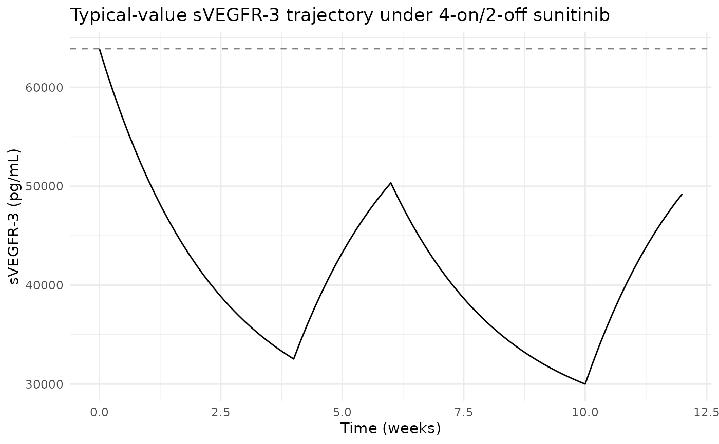
ggplot(sim, aes(time / (7 * 24), circ)) +
  geom_line() +
  geom_hline(yintercept = 4.94, linetype = "dashed", colour = "grey50") +
  labs(x = "Time (weeks)", y = "ANC (10^9/L)",
       title = "Typical-value ANC trajectory") +
  theme_minimal()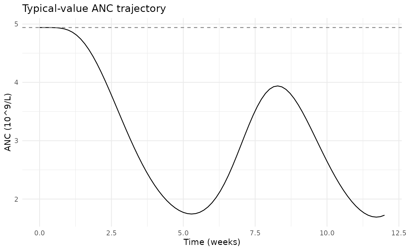
The paper Results: ‘For a typical patient receiving a daily 50-mg sunitinib dose (4/2 schedule) and an ANC0 of 4.94, the model predicted a 62% decrease in ANC corresponding to a nadir of 1.9’. The typical-value simulation here should reproduce this nadir within a factor consistent with the within-cycle integration depth.
Assumptions and deviations
Residual error encoded as linear-scale additive, not Box-Cox. The source Methods state ‘Residual variability was described by an additive (on Box-Cox scale) error model’ with
lambda = 0.2. nlmixr2 / rxode2 do not yet ship a one-line Box-Cox-residual directive; this model file uses a simple linear-scale additive residual SD with the same numeric value (0.406) the paper reports on the Box-Cox-transformed scale. For forward-simulation purposes this is a conservative approximation (the linear-scale variance is larger than the Box-Cox variance at typical ANC values); for re-fitting the user should re-implement the Box-Cox transformation directly.pg.hour/lunit label on ANC EC50. Hansson 2013 Table 2 row ‘ANC EC50’ carries the unit annotation ‘(pg.hour/l)’ (AUC units), but the Methods text identifies the driver of the Emax function as the unitlesssVEGFR-3 REL(relative change in sVEGFR-3 from baseline). The 0.552 value is interpreted here as the unitless sVEGFR-3 REL value at which the drug effect is half-maximal – i.e., when sVEGFR-3 has been depressed by 55.2% below baseline. The(pg.hour/l)annotation in Table 2 appears to be an editing artefact carried over from competing AUC-driven model rows; the in-model EC50 is unitless.Uniform
ktrfor the chain, including circ. The standard Friberg 2002 form uses a single rate constant for the proliferation, transit, and circulating pools, withktr = (n_trans + 1) / MTTandn_trans = 3. Hansson 2013 e85 Methods state that the half-life of circulating neutrophils was fixed to 7 h to enhance physiological interpretation; in this nlmixr2 forward-simulation port the circulating pool sharesktrwith the rest of the chain (matching the standard Friberg form), so the effective circulating-pool half-life isln(2) * MTT / 4= about 43 h withMTT = 248 h. The published MTT and nadir-depth parameters are preserved verbatim; the deviation affects the recovery-shape of the circulating pool but not the on-cycle nadir.Observation name
anc(notCc). The model output is an absolute neutrophil count in 10^9/L, not a drug concentration.checkModelConventions()flags this as anobservationwarning; the deviation is the canonical “non-PK PD output” exemption.Upstream PK and biomarker dependencies. The Houk 2009 sunitinib popPK model (the source of per-subject CLI) is not packaged in nlmixr2lib at extraction time. The upstream Hansson 2013a biomarker model (BAS_SVEGFR3, MRT_SVEGFR3, EC50_SVEGFR3) is packaged but must be simulated separately to get per-subject covariates for realistic IIV simulations. For typical-cohort simulations set every subject to the Hansson_2013a typical values (CLI = 32.819 L/h, BAS_SVEGFR3 = 63 900 pg/mL, MRT_SVEGFR3 = 401 h, EC50_SVEGFR3 = 1.0).
Detailed per-cohort demographics absent. Hansson 2013 e85 Table 1 reports the per-study sample size, dosing schedule, and observed-AE distributions, but the trimmed PDF section that includes Methods + Results + Tables does not carry a baseline-demographics breakdown by cohort (age, weight, sex, race); the model’s
populationmetadata records that gap.