Sunitinib hand-foot syndrome (Hansson 2013)
Source:vignettes/articles/Hansson_2013_sunitinib_hfs.Rmd
Hansson_2013_sunitinib_hfs.RmdModel and source
- Citation: Hansson EK, Ma G, Amantea MA, French J, Milligan PA, Friberg LE, Karlsson MO. PKPD modeling of predictors for adverse effects and overall survival in sunitinib-treated patients with GIST. CPT Pharmacometrics Syst Pharmacol 2013;2(11):e85.
- Article: doi:10.1038/psp.2013.62
- Upstream sVEGFR-3 biomarker dynamics:
Hansson_2013a_sunitinib(DDMODEL00000197, doi:10.1038/psp.2013.61). - Companion fatigue model:
Hansson_2013c_sunitinib(structurally parallel to this HFS model, with fatigue-specific Table 3 parameters).
This vignette extracts the hand-foot syndrome (HFS)
sub-model from the Hansson 2013 e85 framework. The structural form is
identical to Hansson_2013c_sunitinib (the same first-order
Markov + proportional- odds shape with a delayed sVEGFR-3 driver);
parameter values come from the HFS column of Hansson
2013 Table 3 rather than the fatigue column.
Population
303 adults with imatinib-resistant GIST pooled from four sunitinib trials (Demetri 2006, George 2009, Shirao 2010, Maki 2005). HFS grade distribution per study (highest observed severity per subject; Hansson 2013 Table 1): study 1004 (83% grade 0, 5.0% 1, 6.9% 2, 5.4% 3+); study 1047 (100% grade 0); study 1045 (14% grade 0, 20% 1, 34% 2, 31% 3+); study 013 (not available). HFS grade 4 was reported in 0% of patients, so grades 3 and 4 were grouped per Methods.
readModelDb("Hansson_2013_sunitinib_hfs")$population
returns the same information programmatically.
Source trace
All parameter values come from Hansson 2013 e85 Table 3 ‘HFS model’
column. The cumulative-logit parameterisation matches
Hansson_2013c_sunitinib: per starting state, three
baseline-logit population parameters carry the cumulative sums
clge1_px<i> = B1|i,
clge2_px<i> = B1|i + B2|i, and
clge3_px<i> = B1|i + B2|i + B>=3|i. The placebo
slope e_bm_px<i> is applied to a delayed sVEGFR-3
relative-change signal bm (first-order effect compartment
with ke0 = 0.347/h per Results).
| Equation / parameter | Source location |
|---|---|
Eq. 2 logit form P(b\|a) = expit(B + g(x))
|
Methods ‘an extension of the proportional odds model was used to describe … HFS over time’ |
Effect-compartment delay
d/dt(bm) = ke0 * (bm_input - bm)
|
Results: ‘Incorporation of an effect compartment into the model [ke0 = … 0.347/hour (HFS)] significantly improved both the fatigue and HFS models’ |
bm_input = (svegfr3 - BAS_SVEGFR3) / BAS_SVEGFR3 |
Methods ‘relative change over time for sVEGFR-3 (sVEGFR-3 REL)’ |
auc = DOSE / CLI |
Methods (matches Hansson_2013a / 2013c convention) |
clge1_px0 = -10.4 |
Table 3 HFS B1|0 = -10.4 (RSE 11%) |
clge2_px0 = -11.374 = -10.4 + -0.974 |
Table 3 HFS B2|0 = -0.974 (RSE 13%) |
clge3_px0 = -12.964 |
Table 3 HFS B>=3|0 = -1.59 (RSE 19%) |
clge1_px1 = 2.29 |
Table 3 HFS B1|1 = 2.29 (RSE 14%) |
clge2_px1 = -7.24 = 2.29 + -9.53 |
Table 3 HFS B2|1 = -9.53 (RSE 5.0%) |
clge3_px1 = -8.57 |
Table 3 HFS B>=3|1 = -1.33 (RSE 24%) |
clge1_px2 = 3.04 |
Table 3 HFS B1|2 = 3.04 (RSE 15%) |
clge2_px2 = 2.293 = 3.04 + -0.747 |
Table 3 HFS B2|2 = -0.747 (RSE 14%) |
clge3_px2 = -6.797 |
Table 3 HFS B>=3|2 = -9.09 (RSE 5.1%) |
clge1_px3 = 3.4 |
Table 3 HFS B1|>3 = 3.4 (RSE 21%) |
clge2_px3 = 1.75 = 3.4 + -1.65 |
Table 3 HFS B2|>3 = -1.65 (RSE 23%) |
clge3_px3 = 1.297 |
Table 3 HFS B>=3|>=3 = -0.453 (RSE 37%) |
e_bm_px0 = -8.00 |
Table 3 HFS Slope x|0 (RSE 14%) |
e_bm_px1 = -6.00 |
Table 3 HFS Slope x|1 (RSE 18%) |
e_bm_px2 = -3.23 |
Table 3 HFS Slope x|2 (RSE 43%) |
e_bm_px3 = -4.75 |
Table 3 HFS Slope x|>=3 (RSE 32%) |
ke0 = 0.347 (fixed) |
Results: ke0 = 0.347/h for HFS effect compartment |
etaclge_px0 ~ 9.4249 |
Table 3 HFS omega x|0 = 3.07 (variance = 3.07^2) (RSE 67%) |
etaclge_px1 ~ 0.8136 |
Table 3 HFS omega x|1 = 0.902 (RSE 54%) |
etaclge_px2 ~ 0.0729 |
Table 3 HFS omega x|2 = 0.270 (RSE 118%) |
etaclge_px3 ~ fixed(0.0001) |
Table 3 HFS omega x|>=3 = NE (Not Estimated) |
Drug-exposure inputs and required covariates
Same as Hansson_2013c_sunitinib: DOSE (mg,
time-varying), CLI (L/h, per-subject),
BAS_SVEGFR3 (pg/mL), MRT_SVEGFR3 (h),
EC50_SVEGFR3 (mg*h/L). For typical-cohort vignette
simulations use the Hansson 2013a typical values (BAS_SVEGFR3 = 63 900,
MRT_SVEGFR3 = 401, EC50_SVEGFR3 = 1.0, CLI = 32.819).
Virtual cohort
mod  <- readModelDb("Hansson_2013_sunitinib_hfs")
modT <- rxode2::zeroRe(mod)
#> ℹ parameter labels from comments will be replaced by 'label()'

on_off_dose <- function(time_h, daily_mg = 50) {
  week_idx  <- floor(time_h / (7 * 24))
  cycle_idx <- week_idx %% 6
  ifelse(cycle_idx < 4, daily_mg, 0)
}

obs_times <- seq(0, 12 * 7 * 24, by = 24)

events <- data.frame(
  id           = 1L,
  time         = obs_times,
  evid         = 0L,
  amt          = 0,
  cmt          = "svegfr3",
  DOSE         = on_off_dose(obs_times, daily_mg = 50),
  CLI          = 32.819,
  BAS_SVEGFR3  = 63900,
  MRT_SVEGFR3  = 401,
  EC50_SVEGFR3 = 1.0
)

head(events, 6)
#>   id time evid amt     cmt DOSE    CLI BAS_SVEGFR3 MRT_SVEGFR3 EC50_SVEGFR3
#> 1  1    0    0   0 svegfr3   50 32.819       63900         401            1
#> 2  1   24    0   0 svegfr3   50 32.819       63900         401            1
#> 3  1   48    0   0 svegfr3   50 32.819       63900         401            1
#> 4  1   72    0   0 svegfr3   50 32.819       63900         401            1
#> 5  1   96    0   0 svegfr3   50 32.819       63900         401            1
#> 6  1  120    0   0 svegfr3   50 32.819       63900         401            1
Mechanistic-sanity simulation (F.3)
The HFS model is a Markov + proportional-odds modality without a
published NCA table; the F.3 mechanistic-sanity recipe applies.
Typical-value simulation should reproduce sVEGFR-3 depletion under drug,
bm (the effect-compartment-smoothed relative-change signal)
moving negative, and each per-state P(grade >= 1) rising.
sim <- rxode2::rxSolve(modT, events = events) |> as.data.frame()
#> ℹ omega/sigma items treated as zero: 'etaclge_px0', 'etaclge_px1', 'etaclge_px2', 'etaclge_px3'

ggplot(sim, aes(time / (7 * 24), svegfr3)) +
  geom_line() +
  geom_hline(yintercept = 63900, linetype = "dashed", colour = "grey50") +
  labs(x = "Time (weeks)", y = "sVEGFR-3 (pg/mL)",
       title = "Typical-value sVEGFR-3 trajectory under 4-on/2-off sunitinib") +
  theme_minimal()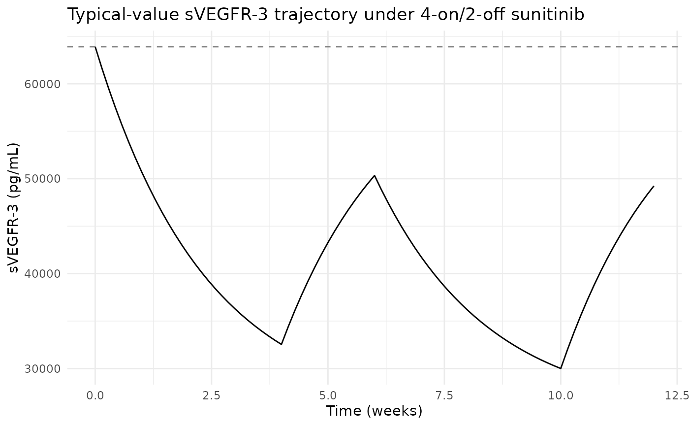
ggplot(sim, aes(time / (7 * 24), bm)) +
  geom_line() +
  geom_hline(yintercept = 0, linetype = "dashed", colour = "grey50") +
  labs(x = "Time (weeks)", y = "bm (delayed sVEGFR-3 relative change)",
       title = "Effect-compartment-smoothed sVEGFR-3 REL signal") +
  theme_minimal()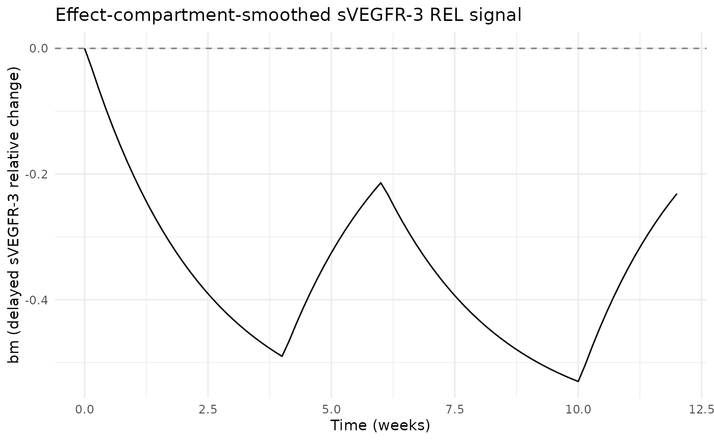
on_cycle_end  <- sim |> dplyr::filter(time == 4 * 7 * 24) |> dplyr::pull(svegfr3)
off_cycle_end <- sim |> dplyr::filter(time == 6 * 7 * 24) |> dplyr::pull(svegfr3)
bl            <- sim |> dplyr::filter(time == 0)         |> dplyr::pull(svegfr3)

stopifnot(on_cycle_end < bl)                                  # drug depletes sVEGFR-3
stopifnot(abs(off_cycle_end - bl) < abs(on_cycle_end - bl))   # off-cycle relaxation

p_grade1_baseline <- sim |> dplyr::filter(time == 0) |> dplyr::pull(pge10)
p_grade1_oncycle  <- sim |> dplyr::filter(time == 4 * 7 * 24) |> dplyr::pull(pge10)
stopifnot(p_grade1_oncycle > p_grade1_baseline)               # drug raises P(HFS>=1)

data.frame(
  metric = c(
    "sVEGFR-3 baseline (pg/mL)",
    "sVEGFR-3 end of first on-cycle (pg/mL)",
    "sVEGFR-3 end of first off-cycle (pg/mL)",
    "P(HFS grade>=1 | prev=0) baseline",
    "P(HFS grade>=1 | prev=0) end of first on-cycle"
  ),
  value = c(
    round(bl, 1),
    round(on_cycle_end, 1),
    round(off_cycle_end, 1),
    round(p_grade1_baseline, 6),
    round(p_grade1_oncycle, 6)
  )
)
#>                                           metric       value
#> 1                      sVEGFR-3 baseline (pg/mL) 63900.00000
#> 2         sVEGFR-3 end of first on-cycle (pg/mL) 32542.10000
#> 3        sVEGFR-3 end of first off-cycle (pg/mL) 50334.10000
#> 4              P(HFS grade>=1 | prev=0) baseline     0.00003
#> 5 P(HFS grade>=1 | prev=0) end of first on-cycle     0.00153
Per-state transition probabilities at typical values
sim_baseline <- sim |> dplyr::filter(time == 0)
P_typical <- with(sim_baseline,
                  rbind(
                    "prev=0"  = c(p00, p10, p20, p30),
                    "prev=1"  = c(p01, p11, p21, p31),
                    "prev=2"  = c(p02, p12, p22, p32),
                    "prev=3+" = c(p03, p13, p23, p33)
                  ))
colnames(P_typical) <- c("next=0", "next=1", "next=2", "next=3+")
round(P_typical, 4)
#>         next=0 next=1 next=2 next=3+
#> prev=0  1.0000 0.0000 0.0000  0.0000
#> prev=1  0.0920 0.9073 0.0005  0.0002
#> prev=2  0.0457 0.0461 0.9072  0.0011
#> prev=3+ 0.0323 0.1158 0.0666  0.7853

stopifnot(all(abs(rowSums(P_typical) - 1) < 1e-9))
The matrix is dominated by the diagonal – subjects tend to stay in
their previous HFS state from visit to visit. The very small
P(grade>=1|prev=0) at baseline (the clge1_px0 = -10.4
typical logit maps to expit(-10.4) ~ 3e-5) reflects the published
Methods finding that HFS development is rare and slow without drug, with
a much higher probability of escalation conditional on already having
grade 1 (clge1_px1 = 2.29 -> expit(2.29) ~ 0.91).
Assumptions and deviations
Cumulative-logit reparameterisation. Same deviation as the companion
Hansson_2013c_sunitinibmodel. The source.modformB1 + B2 + B3withB2 <= 0,B3 <= 0cannot be expressed in nlmixr2’s mu-reference parser without splitting into per-threshold population parameters; this model file uses the equivalent cumulative-logit form. The math is identical at the published parameter values; the cost is that theB2 <= 0/B3 <= 0monotonicity constraint is not enforced at the parameter level (it is honoured at typical-value initialisation).Markov + proportional-odds likelihood not natively expressed. Same deviation as
Hansson_2013c_sunitinib. nlmixr2 / rxode2 do not natively express “previous DV”-conditioned discrete likelihoods, so the model exposes the per-state transition probabilities (p00..p33) as deterministic functions of time and uses a continuous “expected HFS grade given previous = 0” output (hfs_grade) as the formal observation with a placeholder additive residual erroraddSd_hfs_grade = 0.5. The published 0.5 placeholder is not from the source; users fitting the actual likelihood need to extend the model with a per-recordPDVcolumn and a conditional~ ll(...)form outside the scope of this skill.PX3+ IIV fixed at tiny non-zero. Table 3 HFS reports
omega x|>=3 = NE(Not Estimated). The strict source-faithful encoding is a zero-variance random effect, but rxode2 requires positive-definite omega; this model file fixes the PX3+ eta variance at 1e-4 (effectively zero) viaetaclge_px3 ~ fixed(0.0001). For forward simulation this has no observable effect; for re-fitting the user should drop the eta entirely.Effect-compartment ke0 fixed at 0.347/h. Hansson 2013 Results report the HFS effect-compartment rate constant as a point value (
ke0 = 0.347/h) with no uncertainty; wrapped infixed()per parameter-naming guidance.Observation name
hfs_grade(notCc). The model output is an ordinal NCI-CTC grade, not a drug concentration. Same exemption asHansson_2013c_sunitinib(fatigue_grade).Upstream PK and biomarker dependencies. Same as
Hansson_2013c_sunitinib: the Houk 2009 sunitinib popPK (CLI source) is not packaged. The upstream Hansson 2013a biomarker model is packaged but must be simulated separately for IIV-realistic per-subject upstream covariates.