Sunitinib diastolic blood pressure (Hansson 2013)
Source:vignettes/articles/Hansson_2013_sunitinib_dbp.Rmd
Hansson_2013_sunitinib_dbp.RmdModel and source
- Citation: Hansson EK, Ma G, Amantea MA, French J, Milligan PA, Friberg LE, Karlsson MO. PKPD modeling of predictors for adverse effects and overall survival in sunitinib-treated patients with GIST. CPT Pharmacometrics Syst Pharmacol 2013;2(11):e85.
- Article: doi:10.1038/psp.2013.62
- Indirect-response form adapted from Keizer RJ et al. J Pharmacokinet Pharmacodyn 2010;37(4):347-363, doi:10.1007/s10928-010-9163-3.
This vignette extracts the diastolic blood pressure (dBP) sub-model from the Hansson 2013 e85 framework.
Population
303 adults with imatinib-resistant GIST pooled from four sunitinib
trials (Demetri 2006, George 2009, Shirao 2010, Maki 2005); dose range
25-75 mg PO QD on a 4/2, 2/2, 2/1, or continuous schedule. Hansson 2013
Table 1 reports median (range) observed dBP during treatment of 78-80
(20-130) mmHg across studies. The dBP model carries a separately
estimated baseline for placebo-arm subjects (PLACEBO = 1,
dBP0 = 77.6 mmHg) vs active sunitinib (PLACEBO = 0, dBP0 =
71.8 mmHg). Methods note that the actual time of day for blood-pressure
measurements was not available; all observations were assumed to occur
in the morning.
readModelDb("Hansson_2013_sunitinib_dbp")$population
returns the same information programmatically.
Source trace
All parameter values come from Hansson 2013 e85 Table 2 ‘Blood
pressure model’ block. The indirect-response form is the standard
Kin-stimulation shape with kin = dBP0 * kout (so the
drug-free steady state of dBP equals dBP0) and a linear drug effect
(1 + dBP_slope * AUC).
| Equation / parameter | Source location |
|---|---|
| Indirect-response with Kin stimulation | Methods ‘Sunitinib AUC was linked to the production rate (Kin) by a linear slope factor (dBP Drug effect)’ |
kin = dbp0 * kout |
Methods ‘Kin was derived as dBP0 x kout’ |
drug_effect = 1 + dBP_slope * AUC |
Methods ‘a linear slope factor (dBP Drug effect)’ |
auc = DOSE / CLI |
Methods ‘Sunitinib AUC was linked to the production rate’ (matches Hansson_2013a / 2013c convention) |
ldbp0 = log(71.8) mmHg |
Table 2 row ‘dBP0’ = 71.8 (RSE 1.0%) |
e_placebo_dbp0 = log(77.6 / 71.8) = 0.0777 |
Table 2 row ‘dBP0 placebo’ = 77.6 (RSE 1.6%) |
lmrt = log(361) h |
Table 2 row ‘MRT (= 1/kout)’ = 361 h (RSE 17%) |
ldbp_slope = log(0.119) L/(mg*h) |
Table 2 row ‘dBP slope’ = 0.119 (RSE 9.4%) |
etaldbp0 + etaldbp_slope ~ c(0.01435, 0.04657, 0.3578) |
Table 2 IIV CV% (dBP0 = 12%, dBP_slope = 65%), Results: ‘A correlation between dBP0 and dBP Drug effect (65%) was estimated’ |
etalmrt ~ 0.5328 |
Table 2 IIV CV% MRT = 83% |
addSd_dbp = 6.24 mmHg |
Table 2 row ‘Residual error (mmHg)’ = 6.24 (RSE 16%) |
propSd_dbp = 0.0697 |
Table 2 row ‘Residual error (%)’ = 6.97 (RSE 24%) |
Drug-exposure inputs and required covariates
-
DOSE(mg) – time-varying daily sunitinib dose; 0 mg during off-cycles or placebo. -
CLI(L/h) – per-subject sunitinib clearance; typical 32.819 L/h. -
PLACEBO(0/1) – 1 for placebo-arm subjects (Study 1004 placebo run-in); switches the typical baseline dBP0 from 71.8 to 77.6 mmHg.
Virtual cohort
mod  <- readModelDb("Hansson_2013_sunitinib_dbp")
modT <- rxode2::zeroRe(mod)
#> ℹ parameter labels from comments will be replaced by 'label()'

on_off_dose <- function(time_h, daily_mg = 50) {
  week_idx  <- floor(time_h / (7 * 24))
  cycle_idx <- week_idx %% 6
  ifelse(cycle_idx < 4, daily_mg, 0)
}

# 12-week typical-cohort simulation; daily observations.
obs_times <- seq(0, 12 * 7 * 24, by = 24)

events <- data.frame(
  id      = 1L,
  time    = obs_times,
  evid    = 0L,
  amt     = 0,
  cmt     = "dbp",
  DOSE    = on_off_dose(obs_times, daily_mg = 50),
  CLI     = 32.819,
  PLACEBO = 0
)

head(events, 6)
#>   id time evid amt cmt DOSE    CLI PLACEBO
#> 1  1    0    0   0 dbp   50 32.819       0
#> 2  1   24    0   0 dbp   50 32.819       0
#> 3  1   48    0   0 dbp   50 32.819       0
#> 4  1   72    0   0 dbp   50 32.819       0
#> 5  1   96    0   0 dbp   50 32.819       0
#> 6  1  120    0   0 dbp   50 32.819       0
Mechanistic-sanity simulation (F.3)
The paper Results: ‘The final model predicted a drug-induced increase in dBP by 10 mmHg for the typical patient with a baseline dBP of 71.8 mmHg treated with 50 mg sunitinib receiving a 4/2 schedule.’ The typical-value simulation should reproduce a near-10 mmHg rise during on-cycle steady state and a return towards baseline during off-cycle.
sim <- rxode2::rxSolve(modT, events = events) |> as.data.frame()
#> ℹ omega/sigma items treated as zero: 'etaldbp0', 'etaldbp_slope', 'etalmrt'

ggplot(sim, aes(time / (7 * 24), dbp)) +
  geom_line() +
  geom_hline(yintercept = 71.8, linetype = "dashed", colour = "grey50") +
  labs(x = "Time (weeks)", y = "dBP (mmHg)",
       title = "Typical-value dBP trajectory under 4-on/2-off sunitinib (active arm)") +
  theme_minimal()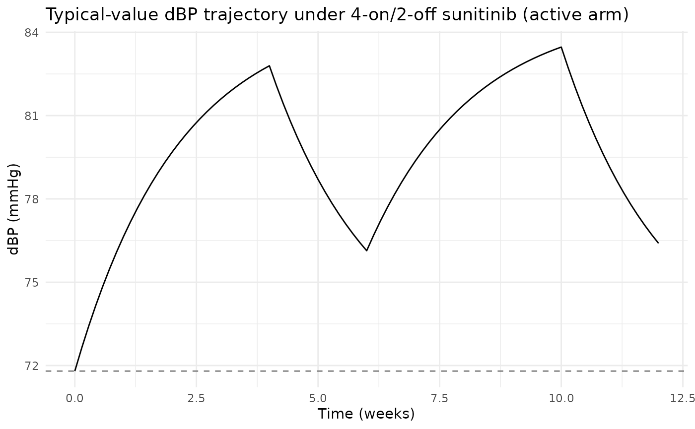
end_on_cycle  <- sim$dbp[sim$time == 4 * 7 * 24]
end_off_cycle <- sim$dbp[sim$time == 6 * 7 * 24]
baseline_dbp  <- sim$dbp[sim$time == 0]

data.frame(
  metric = c("baseline (typical)", "end of first on-cycle", "end of first off-cycle"),
  dbp_mmHg = c(round(baseline_dbp, 2), round(end_on_cycle, 2), round(end_off_cycle, 2)),
  delta_vs_baseline = c(0, round(end_on_cycle - baseline_dbp, 2), round(end_off_cycle - baseline_dbp, 2))
)
#>                   metric dbp_mmHg delta_vs_baseline
#> 1     baseline (typical)    71.80              0.00
#> 2  end of first on-cycle    82.79             10.99
#> 3 end of first off-cycle 76.13 4.33Placebo-arm comparison
events_pla <- transform(events, DOSE = 0, PLACEBO = 1)
sim_pla    <- rxode2::rxSolve(modT, events = events_pla) |> as.data.frame()
#> ℹ omega/sigma items treated as zero: 'etaldbp0', 'etaldbp_slope', 'etalmrt'

ggplot() +
  geom_line(data = sim,     aes(time / (7 * 24), dbp, colour = "Active 50 mg 4/2"), linewidth = 0.7) +
  geom_line(data = sim_pla, aes(time / (7 * 24), dbp, colour = "Placebo arm"), linewidth = 0.7) +
  geom_hline(yintercept = 71.8, linetype = "dashed", colour = "grey50") +
  geom_hline(yintercept = 77.6, linetype = "dashed", colour = "grey50") +
  scale_colour_manual(values = c("Active 50 mg 4/2" = "#1f77b4", "Placebo arm" = "#ff7f0e")) +
  labs(x = "Time (weeks)", y = "dBP (mmHg)", colour = NULL,
       title = "Treated vs placebo dBP trajectories (typical values)") +
  theme_minimal()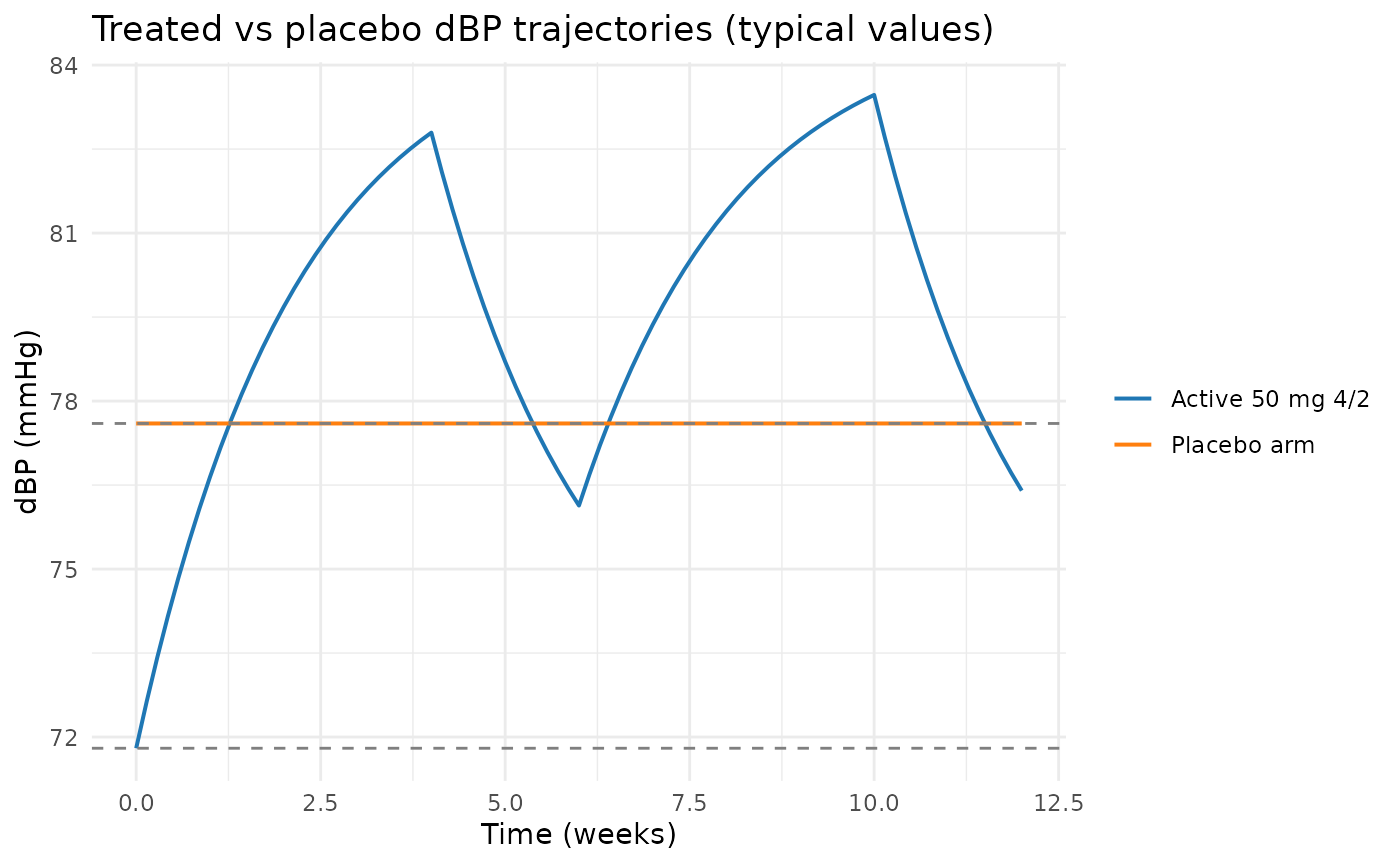
Assumptions and deviations
Observation name
dbp(notCc). The model output is diastolic blood pressure in mmHg, not a drug concentration.checkModelConventions()flags this as anobservationwarning; the deviation is the canonical “non-PK PD output” exemption.Concentration-units field.
units$concentrationis set to"mmHg (diastolic blood pressure)"rather than a mass/volume string because the modality is a physiological measurement.checkModelConventions()flags this as aunitswarning.Upstream PK dependency. The Houk 2009 sunitinib popPK model (the source of per-subject CLI) is not packaged in nlmixr2lib at extraction time. For typical-cohort simulations set every subject to
CLI = 32.819 L/h.Detailed per-cohort demographics absent. Hansson 2013 e85 Table 1 reports per-study sample size and dosing schedule but the trimmed PDF section does not include a baseline-demographics breakdown by cohort (age, weight, sex, race); the model’s
populationmetadata records that gap.