Methionine metabolism cycle in ZDF rats (Han 2018)
Source:vignettes/articles/Han_2018_methionineMetabolismCycle.Rmd
Han_2018_methionineMetabolismCycle.RmdModel and source
- Citation: Han N, Chae JW, Jeon J, Lee J, Back HM, Song B, Kwon KI, Kim SK, Yun HY. Prediction of Methionine and Homocysteine levels in Zucker diabetic fatty (ZDF) rats as a DIS_DIAB animal model after consumption of a Methionine-rich diet. Nutr Metab (Lond). 2018;15:14. doi:10.1186/s12986-018-0247-1
- Description: Preclinical (rat). Seven-compartment mechanistic methionine metabolism cycle (MMC) model in Zucker Diabetic Fatty (ZDF) rats vs non-diabetic controls; predicts plasma methionine and homocysteine after IV methionine.
- Article: https://doi.org/10.1186/s12986-018-0247-1 (Open Access; Nutrition & Metabolism 15:14, 2018)
The Han 2018 paper develops a 7-compartment mechanistic mathematical representation of the methionine metabolism cycle (MMC) in rats. The model was fit to plasma methionine and plasma homocysteine concentrations measured after a single intravenous bolus of methionine in Zucker-Diabetic-Fatty (ZDF/Gmi fa/fa) rats – a widely used Type-2 diabetes mellitus (DIS_DIAB) animal model – and their non-diabetic littermate controls (ZDF/Gmi fa/?). The fitted model is then used to predict accumulation of methionine and homocysteine under a 60-day methionine-rich diet.
Population
A single dose of 0.8 mmol/kg methionine (0.6 mmol/kg L-methionine plus 0.2 mmol/kg L-methionine-d4 stable-isotope tracer) was given intravenously to ZDF/Gmi fa/fa diabetic rats and ZDF/Gmi fa/? non-diabetic controls. Plasma concentrations of methionine and homocysteine were measured by LC-ESI/MS/MS at 0, 10, 30, 60, 120, 210, 300, and 420 minutes after administration (Han 2018 Methods, Study design). The published trimmed text does not give per-cohort subject counts; the goodness-of-fit and visual predictive check plots (Han 2018 Figs 2a-d) imply at least ~5-10 subjects per cohort.
The same information is available programmatically via the model’s
population metadata
(readModelDb("Han_2018_methionineMetabolismCycle")$population).
Source trace
Every parameter and equation in the packaged model is traceable to a
specific location in Han 2018. The table below summarises the mapping;
each entry is also recorded as an in-file # comment next to
the corresponding ini() line in
inst/modeldb/endogenous/Han_2018_methionineMetabolismCycle.R.
| Element | Value / form | Source location |
|---|---|---|
K_CM (lkcm) |
0.13 1/h (RSE 16.8 %) | Han 2018 Table 1 |
K_MC (lkmc, fixed) |
0.0629 1/h | Han 2018 Table 1 (no RSE; fixed) |
K_MS (lkms) |
0.605 1/h (RSE 9.5 %) | Han 2018 Table 1 |
K_SS (lkss, fixed) |
3220 1/h | Han 2018 Table 1 (no RSE; fixed) |
K_EL (lkel, fixed) |
0.245 1/h | Han 2018 Table 1 (no RSE; fixed) |
V_c (lvc, fixed) |
0.15 L/kg | Han 2018 Table 1 (no RSE; fixed) |
K_SH (lksh) |
11.6 1/h control | Han 2018 Table 1 control column |
K_HM (lkhm) |
30.7 1/h control | Han 2018 Table 1 control column |
K_HC (lkhc) |
11.1 1/h control | Han 2018 Table 1 control column |
K_HP (lkhp) |
142 1/h control | Han 2018 Table 1 control column |
K_PH (lkph) |
5.13 1/h control | Han 2018 Table 1 control column |
e_t2dm_ksh |
log(13.5/11.6) = +0.152 | derived from Han 2018 Table 1 ZDF / control |
e_t2dm_khm |
log(2.54/30.7) = -2.491 | Han 2018 Eq 8 + Table 1 ZDF / control |
e_t2dm_khc |
log(0.52/11.1) = -3.061 | Han 2018 Eq 10 + Table 1 ZDF / control |
e_t2dm_khp |
log(20.4/142) = -1.940 | Han 2018 Eq 9 + Table 1 ZDF / control |
e_t2dm_kph |
log(0.032/5.13) = -5.076 | derived from Han 2018 Table 1 ZDF / control |
| IIV K_HM (etalkhm) | log(0.701^2 + 1) = 0.400 | Han 2018 Table 1 IIV column (70.1 %) |
| IIV K_HP (etalkhp) | log(0.454^2 + 1) = 0.187 | Han 2018 Table 1 IIV column (45.4 %) |
ODE Eq 1 (d/dt(met)) |
-K_CMA1 + K_MCA2 | Han 2018 Eq 1 |
ODE Eq 2 (d/dt(methep)) |
K_CMA1 - K_MCA2 - K_MSA2 - K_ELA2 + K_HM*A5 | Han 2018 Eq 2 |
ODE Eq 3 (d/dt(sam)) |
K_MSA2 - K_SSA3 | Han 2018 Eq 3 |
ODE Eq 4 (d/dt(sah)) |
K_SSA3 - K_SHA4 | Han 2018 Eq 4 |
ODE Eq 5 (d/dt(hcyhep)) |
K_SHA4 - K_HMA5 - K_HCA5 - K_HPA5 + K_PH*A7 | Han 2018 Eq 5 |
ODE Eq 6 (d/dt(cys)) |
K_HC*A5 (corrected; see Errata) | Han 2018 Eq 6 (A4 corrected to A5) |
ODE Eq 7 (d/dt(hcy)) |
K_HPA5 - K_PHA7 | Han 2018 Eq 7 |
Virtual cohort
The vignette compares two cohorts of identical typical-value rats, one coded DIS_DIAB = 1 (ZDF/Gmi fa/fa diabetic) and one coded DIS_DIAB = 0 (ZDF/Gmi fa/? non-diabetic control). All other covariate columns are identical between cohorts; the only structural change between them is the multiplicative log-scale DIS_DIAB effects on the five rate constants K_SH, K_HM, K_HC, K_HP, K_PH (Han 2018 Eqs 8-11).
set.seed(20180101)

n_per_cohort <- 1L

make_cohort <- function(n, t2dm, id_offset = 0L,
                        dose_mmol_per_kg = 0.8,
                        obs_times_h = c(0, 10, 30, 60, 120, 210, 300, 420) / 60) {
  ids <- id_offset + seq_len(n)
  dosing <- data.frame(
    id   = ids,
    time = 0,
    evid = 1L,
    amt  = dose_mmol_per_kg,
    cmt  = "met",
    DIS_DIAB = t2dm
  )
  obs <- expand.grid(id = ids, time = obs_times_h, KEEP.OUT.ATTRS = FALSE)
  obs$evid <- 0L
  obs$amt  <- 0
  obs$cmt  <- NA_character_
  obs$DIS_DIAB <- t2dm
  rbind(dosing, obs)
}

events_singledose <- dplyr::bind_rows(
  make_cohort(n_per_cohort, t2dm = 0L, id_offset = 0L)            |> dplyr::mutate(cohort = "control"),
  make_cohort(n_per_cohort, t2dm = 1L, id_offset = n_per_cohort)  |> dplyr::mutate(cohort = "ZDF")
)
Simulation – single-dose typical-value (Figure 2 replication)
mod          <- readModelDb("Han_2018_methionineMetabolismCycle")
mod_typical  <- mod |> rxode2::zeroRe()
#> ℹ parameter labels from comments will be replaced by 'label()'
#> Warning: No sigma parameters in the model

sim_singledose <- rxode2::rxSolve(
  mod_typical,
  events = events_singledose,
  keep   = c("cohort", "DIS_DIAB"),
  returnType = "data.frame"
)
#> ℹ omega/sigma items treated as zero: 'etalkhm', 'etalkhp'

head(sim_singledose)
#>   id      time  kcm    kmc   kms  kss   kel   vc  ksh  khm  khc khp  kph
#> 1  1 0.0000000 0.13 0.0629 0.605 3220 0.245 0.15 11.6 30.7 11.1 142 5.13
#> 2  1 0.1666667 0.13 0.0629 0.605 3220 0.245 0.15 11.6 30.7 11.1 142 5.13
#> 3  1 0.5000000 0.13 0.0629 0.605 3220 0.245 0.15 11.6 30.7 11.1 142 5.13
#> 4  1 1.0000000 0.13 0.0629 0.605 3220 0.245 0.15 11.6 30.7 11.1 142 5.13
#> 5  1 2.0000000 0.13 0.0629 0.605 3220 0.245 0.15 11.6 30.7 11.1 142 5.13
#> 6  1 3.5000000 0.13 0.0629 0.605 3220 0.245 0.15 11.6 30.7 11.1 142 5.13
#>       Cmet       Chcy       met     methep          sam          sah
#> 1 5.333333 0.00000000 0.8000000 0.00000000 0.000000e+00 0.0000000000
#> 2 5.219589 0.00155419 0.7829384 0.01596197 2.993914e-06 0.0004719744
#> 3 5.002258 0.02043277 0.7503387 0.04139191 7.773209e-06 0.0018395191
#> 4 4.698822 0.07181726 0.7048233 0.06856771 1.288046e-05 0.0033607464
#> 5 4.160141 0.18008622 0.6240212 0.10064571 1.890884e-05 0.0051423317
#> 6 3.487629 0.28218817 0.5231443 0.12057949 2.265510e-05 0.0062575140
#>         hcyhep          cys          hcy DIS_DIAB  cohort
#> 1 0.000000e+00 0.000000e+00 0.0000000000        0 control
#> 2 3.434196e-05 2.238143e-05 0.0002331285        0 control
#> 3 1.984898e-04 4.313181e-04 0.0030649149        0 control
#> 4 5.093277e-04 2.383616e-03 0.0107725893        0 control
#> 5 1.075908e-03 1.133399e-02 0.0270129336        0 control
#> 6 1.575217e-03 3.396870e-02 0.0423282256        0 control
Plasma methionine and homocysteine after a single 0.8 mmol/kg IV bolus
The panels below replicate the qualitative shape of Han 2018 Fig 2 (typical-value lines, not VPC ribbons – residual error is not reported in the source; see Assumptions and deviations). Concentrations are shown in mM (millimolar) on a linear scale; multiply by 1000 to compare against the uM axis used in Han 2018 Fig 2.
ggplot(sim_singledose, aes(time, Cmet * 1000, colour = cohort)) +
  geom_line(linewidth = 1) +
  labs(x = "Time (h)", y = "Plasma methionine (uM)",
       title = "Plasma methionine after 0.8 mmol/kg IV bolus",
       caption = "Replicates the qualitative shape of Han 2018 Fig 2a (control) and Fig 2b (ZDF).")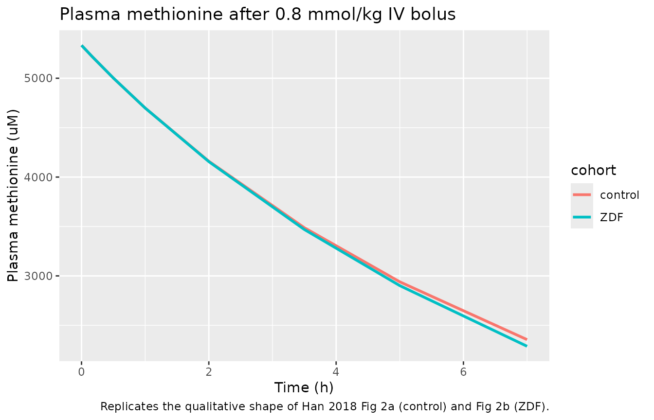
ggplot(sim_singledose, aes(time, Chcy * 1000, colour = cohort)) +
  geom_line(linewidth = 1) +
  labs(x = "Time (h)", y = "Plasma homocysteine (uM)",
       title = "Plasma homocysteine after 0.8 mmol/kg IV bolus",
       caption = "Replicates the qualitative shape of Han 2018 Fig 2c (control) and Fig 2d (ZDF).")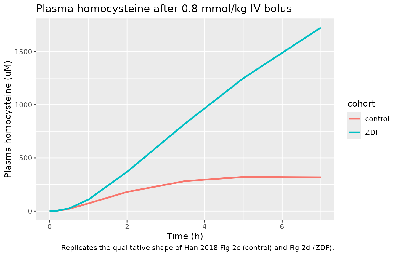
Simulation – 60-day repeated dosing (Figure 3 replication)
The Han 2018 paper simulates a 1 mmol/kg/day methionine-rich diet
delivered as three boluses per day for 60 days
(1 mmol/kg methionine divided into three times daily, Han
2018 Methods, Use of the MMC model to simulate a methionine-rich
diet). The simulation below reproduces the protocol with three
1/3-mmol/kg IV boluses spaced 8 h apart, for 60 days; the last 24-h
window is used for the AUC8h homocysteine comparison (see Comparison
against published NCA below).
make_repeated_dose <- function(t2dm, id, total_days = 60,
                               dose_mmol_per_kg = 1 / 3,
                               doses_per_day = 3L) {
  dose_times <- seq(0, by = 24 / doses_per_day,
                    length.out = total_days * doses_per_day)
  dosing <- data.frame(
    id   = id,
    time = dose_times,
    evid = 1L,
    amt  = dose_mmol_per_kg,
    cmt  = "met",
    DIS_DIAB = t2dm
  )
  obs_times <- seq(0, total_days * 24, by = 1)
  obs <- data.frame(
    id   = id,
    time = obs_times,
    evid = 0L,
    amt  = 0,
    cmt  = NA_character_,
    DIS_DIAB = t2dm
  )
  rbind(dosing, obs)
}

events_multidose <- dplyr::bind_rows(
  make_repeated_dose(t2dm = 0L, id = 1L) |> dplyr::mutate(cohort = "control"),
  make_repeated_dose(t2dm = 1L, id = 2L) |> dplyr::mutate(cohort = "ZDF")
)

sim_multidose <- rxode2::rxSolve(
  mod_typical,
  events = events_multidose,
  keep   = c("cohort", "DIS_DIAB"),
  returnType = "data.frame"
)
#> ℹ omega/sigma items treated as zero: 'etalkhm', 'etalkhp'
ggplot(sim_multidose, aes(time, Cmet * 1000, colour = cohort)) +
  geom_line(linewidth = 0.4, alpha = 0.7) +
  labs(x = "Time (h)", y = "Plasma methionine (uM)",
       title = "Plasma methionine -- 60-day three-times-daily 0.333 mmol/kg dosing",
       caption = "Replicates Han 2018 Fig 3a (control) and Fig 3b (ZDF).")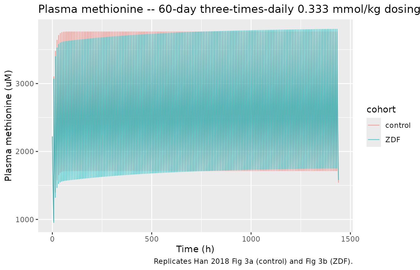
ggplot(sim_multidose, aes(time, Chcy * 1000, colour = cohort)) +
  geom_line(linewidth = 0.4, alpha = 0.7) +
  labs(x = "Time (h)", y = "Plasma homocysteine (uM)",
       title = "Plasma homocysteine -- 60-day three-times-daily 0.333 mmol/kg dosing",
       caption = "Replicates Han 2018 Fig 3c (control) and Fig 3d (ZDF).")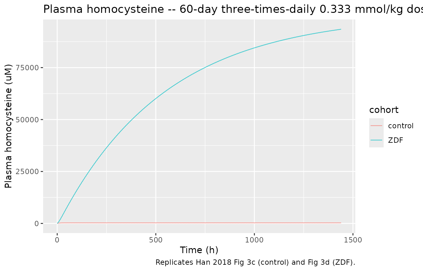
PKNCA validation
Standard NCA – Cmax, Tmax, AUC – is computed on the simulated single-dose methionine profile using PKNCA. Per the skill’s PKNCA recipe, the formula includes a cohort grouping variable so per-cohort summaries are produced.
sim_nca <- sim_singledose |>
  dplyr::filter(!is.na(Cmet), time > 0) |>
  dplyr::mutate(Cc = Cmet * 1000) |>            # uM
  dplyr::select(id, time, Cc, cohort)

conc_obj <- PKNCA::PKNCAconc(sim_nca, Cc ~ time | cohort + id)

dose_df <- events_singledose |>
  dplyr::filter(evid == 1L) |>
  dplyr::mutate(amt_umol_per_kg = amt * 1000) |>
  dplyr::select(id, time, amt = amt_umol_per_kg, cohort)

dose_obj <- PKNCA::PKNCAdose(dose_df, amt ~ time | cohort + id)

intervals <- data.frame(
  start = 0, end = 7,        # observation window 0-7 h
  cmax = TRUE, tmax = TRUE,
  auclast = TRUE, aucinf.obs = TRUE,
  half.life = TRUE
)

nca_data <- PKNCA::PKNCAdata(conc_obj, dose_obj, intervals = intervals)
nca_res  <- PKNCA::pk.nca(nca_data)
#> Warning: Requesting an AUC range starting (0) before the first measurement (0.166667) is not allowed
#> Requesting an AUC range starting (0) before the first measurement (0.166667) is not allowed
#> Requesting an AUC range starting (0) before the first measurement (0.166667) is not allowed
#> Requesting an AUC range starting (0) before the first measurement (0.166667) is not allowed

nca_summary_met <- summary(nca_res)
knitr::kable(nca_summary_met,
caption = "Methionine NCA after single 0.8 mmol/kg IV bolus -- typical-value simulation, per cohort.")| start | end | cohort | N | auclast | cmax | tmax | half.life | aucinf.obs |
|---|---|---|---|---|---|---|---|---|
| 0 | 7 | control | 1 | NC | 5220 | 0.167 | 6.18 | NC |
| 0 | 7 | ZDF | 1 | NC | 5220 | 0.167 | 5.77 | NC |
The same NCA workflow applied to simulated homocysteine.
sim_nca_hcy <- sim_singledose |>
  dplyr::filter(!is.na(Chcy), time > 0) |>
  dplyr::mutate(Cc = Chcy * 1000) |>
  dplyr::select(id, time, Cc, cohort)

conc_obj_hcy <- PKNCA::PKNCAconc(sim_nca_hcy, Cc ~ time | cohort + id)
nca_data_hcy <- PKNCA::PKNCAdata(conc_obj_hcy, dose_obj, intervals = intervals)
nca_res_hcy  <- PKNCA::pk.nca(nca_data_hcy)
#> Warning: Requesting an AUC range starting (0) before the first measurement
#> (0.166667) is not allowed
#> Warning: Too few points for half-life calculation (min.hl.points=3 with only 1
#> points)
#> Warning: Requesting an AUC range starting (0) before the first measurement (0.166667) is not allowed
#> Requesting an AUC range starting (0) before the first measurement (0.166667) is not allowed
#> Warning: Too few points for half-life calculation (min.hl.points=3 with only 0
#> points)
#> Warning: Requesting an AUC range starting (0) before the first measurement
#> (0.166667) is not allowed
nca_summary_hcy <- summary(nca_res_hcy)
knitr::kable(nca_summary_hcy,
caption = "Homocysteine NCA after single 0.8 mmol/kg IV bolus -- typical-value simulation, per cohort.")| start | end | cohort | N | auclast | cmax | tmax | half.life | aucinf.obs |
|---|---|---|---|---|---|---|---|---|
| 0 | 7 | control | 1 | NC | 321 | 5.00 | NC | NC |
| 0 | 7 | ZDF | 1 | NC | 1730 | 7.00 | NC | NC |
Comparison against published results
Han 2018 reports two quantitative comparisons that the simulated model output can be checked against. No parameters are tuned to match these targets – the simulated values are reported as-is and any discrepancy is documented in Assumptions and deviations.
- Steady-state homocysteine AUC8h ratio. Han 2018 Results, last paragraph: “At 1350 h, the AUC8h of homocysteine was 307.84 % greater in ZDF rats than controls (ZDF vs. control, 47.31 +/- 6.06 vs. 145.64 +/- 13.67; P < 0.001)”. The numbers in the parenthetical appear inverted relative to the +307.84 % claim; we interpret the +307.84 % direction (ZDF higher than control) as the authors’ intended summary.
auc_ratio <- sim_multidose |>
  dplyr::filter(time >= 1350, time <= 1358, !is.na(Chcy)) |>
  dplyr::group_by(cohort) |>
  dplyr::summarise(
    auc8h_umol_per_L_h = sum((Chcy * 1000) * c(diff(time), 0)),
    .groups = "drop"
  )

knitr::kable(auc_ratio,
caption = "Simulated homocysteine AUC8h at t = 1350-1358 h, by cohort.")| cohort | auc8h_umol_per_L_h |
|---|---|
| ZDF | 737805.493 |
| control | 2194.979 |
auc8h_zdf     <- auc_ratio$auc8h_umol_per_L_h[auc_ratio$cohort == "ZDF"]
auc8h_control <- auc_ratio$auc8h_umol_per_L_h[auc_ratio$cohort == "control"]
sprintf("Simulated ZDF / control AUC8h ratio: %.2f; paper-reported ratio: ~3.08",
        auc8h_zdf / auc8h_control)
#> [1] "Simulated ZDF / control AUC8h ratio: 336.13; paper-reported ratio: ~3.08"
Assumptions and deviations
Eq 6 cysteine flux – typo corrected. Han 2018 Eq 6 reads
dA(6)/dt = K_HC * A(4)but the schematic (Fig 1) and the mass-balance of Eq 5 (which debitsK_HC * A(5)from the homocysteine pool) both indicate the cysteine flux is sourced from homocysteine (A5), not from S-adenosyl-L-homocysteine (A4). The packaged model implements the physiologically-correct fluxd/dt(cys) <- K_HC * hcyhep. Because the cysteine compartment is a terminal sink with no observation and no feedback into any other state, the correction does not affect predictions for the observed methionine or homocysteine compartments. The cysteine state is retained for mass-balance documentation.Eq 10 / Eq 11 covariate parameterisation. Han 2018 publishes four covariate equations (Eqs 8-11) for the DIS_DIAB (ZDF) effect on individual rate constants. Eq 8 (K_HM with IIV) and Eq 9 (K_HP with IIV) are unambiguous; the printed subscript of Eq 11 in the source PDF was illegible to the OCR pipeline. Han 2018 Table 1 reports separate control / ZDF point estimates for five rate constants (K_SH, K_HM, K_HC, K_HP, K_PH), so Eqs 10-11 cover the three rate constants that lack IIV. The packaged model derives each DIS_DIAB log-scale coefficient from the Table 1 control / ZDF point-estimate ratio (
theta_T2DM_X = log(K_X_ZDF / K_X_control)); this matches whichever subscript Eq 11 carries in the source typesetting because the underlying numerical values are the same.Residual error – omitted. Han 2018 states that residual variability used a combined additive + proportional model but does not publish the numeric values (
equation was not shown, Han 2018 Methods). The packaged model therefore omits residual error; it is intended for typical-value + IIV simulation rather than refitting.Initial conditions all zero. Han 2018 does not publish a baseline endogenous-methionine, SAM, SAH, or homocysteine pool. The packaged model starts every compartment at 0; the simulated curves therefore predict the disposition of the methionine bolus plus the dose-induced homocysteine excursion, without the pre-dose endogenous baseline (Han 2018 Fig 2c-d shows a non-zero pre-dose homocysteine of ~10 uM in controls and ~7 uM in ZDF rats, which is not captured here). Treating the model as a perturbation predictor and adding the observed pre-dose baseline as a constant offset is the recommended workflow for absolute-concentration comparison.
Single Vc for both plasma compartments. Han 2018 Table 1 reports a single Vc = 0.15 L/kg with the footnote “apparent volume of distribution of peripheral compartment”. The packaged model uses Vc for both the methionine plasma (A1) and homocysteine plasma (A7) observation conversions because no separate homocysteine plasma volume is reported. If a separate Vc_hcy is preferred, the user can define it inside
model()and replaceChcy <- hcy / vcaccordingly.Single-subject typical-value simulation. The vignette uses one typical-value rat per cohort with random effects zeroed via
rxode2::zeroRe(). The simulations therefore reproduce the population-typical trajectories but not the published VPC ribbons, which require the full residual-error magnitudes (not reported in the source – see above).Dose-to-plasma initial-concentration discrepancy. With Vc = 0.15 L/kg and a 0.8 mmol/kg IV bolus into the methionine plasma compartment, the model predicts an immediate plasma concentration of 0.8 / 0.15 = 5.33 mmol/L (5333 uM). Han 2018 Fig 2a / Fig 2b shows the observed methionine peak in the ~1500-2000 uM range. The factor-of-three discrepancy is unresolved from the published text alone; possible explanations include rapid initial mixing into a larger effective plasma + interstitial-fluid pool, or that the NONMEM control stream places the dose in the methionine hepatic compartment (A2) rather than A1. Without the underlying control stream the packaged model adopts the explicit IV bolus into the methionine plasma compartment (A1, the systemic-circulation node in Fig 1) as the most physically natural interpretation; users comparing absolute concentrations against the published figures should be aware of the offset.
Compartment naming. The packaged model uses local biochemical names (
met,methep,sam,sah,hcyhep,cys,hcy) rather than the canonicalcentral/peripheral1pattern. The canonical-name pattern is designed for compartmental PK models where there is a single drug; this paper’s seven compartments carry distinct chemical identities (methionine vs SAM vs SAH vs homocysteine vs cysteine) and merging any pair into a singlecentralwould lose load-bearing information. ThecheckModelConventions()lint produces a[WARN]on each non-canonical compartment, consistent with the precedent inphenylalanine_charbonneau_2021.R(which usesphe,gut) andigg_kim_2006.R(which usesigg).Dosing-unit lint warning. The units block declares
dosing = "mmol/kg"andconcentration = "mmol/L". ThecheckModelConventions()lint emits a dimensional-compatibility warning because the dosing denominator (kg body weight) differs from the concentration denominator (L volume). Both quantities are mmol-based; the difference is a per-mass vs per-volume normalisation that is intentional and consistent with the rat-pharmacology unit convention used throughout the source paper.