PSA kinetics and survival in mCRPC (Desmee 2015)
Source:vignettes/articles/Desmee_2015_PSA_mCRPC.Rmd
Desmee_2015_PSA_mCRPC.RmdModel and source
- Citation: Desmee S, Mentre F, Veyrat-Follet C, Guedj J. Nonlinear mixed-effect models for prostate-specific antigen kinetics and link with survival in the context of metastatic prostate cancer: a comparison by simulation of two-stage and joint approaches. AAPS J. 2015 May;17(3):691-9. doi:10.1208/s12248-015-9745-5. Simulation parameter values inspired from one arm of the VENICE phase III trial (Tannock IF et al., Lancet Oncol. 2013;14:760-8; doi:10.1016/S1470-2045(13)70184-0).
- Description: Mechanistic joint biomarker-survival model for prostate-specific antigen (PSA) kinetics under chemotherapy in metastatic castration-resistant prostate cancer (mCRPC). PSA is produced by a proliferating prostate-cell compartment and eliminated by a first-order process; chemotherapy blocks cell proliferation at a per-subject effectiveness eps until an individual escape time Tesc. The Weibull-baseline overall-survival hazard is log-linear in the current PSA value. This is a published-simulation-study model: parameter VALUES are pre-specified (inspired by one arm of the Tannock 2013 VENICE phase III trial), not estimated from real-data fits.
- Article: AAPS J. 2015 May;17(3):691-9
This is a published simulation study, not a real-data fit. The mechanistic PSA-kinetics model was proposed by Desmee et al. and the parameter values were chosen to mimic one arm of the Tannock 2013 VENICE phase III trial in metastatic castration-resistant prostate cancer (mCRPC). The original purpose of the paper was to evaluate, by simulation, the SAEM algorithm in Monolix for fitting nonlinear-biomarker joint models against three estimation alternatives (two-stage, joint sequential, full joint). Here we focus on reproducing the data-generating model.
Population and design
The simulation cohort is M = 100 datasets x N = 500 patients. PSA observations are scheduled every 3 weeks for 2 years (max 36 observations per subject) and follow-up is censored at t = 735 days. The only mechanism for dropout is death.
Four survival scenarios were considered (Table II of the source paper):
| Scenario | beta | lambda (day) | k | Notes |
|---|---|---|---|---|
| No link | 0.000 | 580 | 1.5 | PSA does not enter the hazard |
| Low link | 0.005 | 765 | 1.5 | Weak PSA-survival association |
| High link | 0.020 | 2150 | 1.5 | Strong association; canonical scenario in this file |
| Short survival | 0.020 | 580 | 1.5 | Strong association + high baseline risk |
lambda was calibrated in each scenario so that median
end-of-study survival (at t = 735 day) was ~25% under the median
PSA-kinetic parameters (r = 0.05, PSA0 = 80, eps = 0.3, Tesc = 140). The
packaged model in
inst/modeldb/therapeuticArea/oncology/Desmee_2015_PSA_mCRPC.R
ships the High link scenario as its default; the
vignette below replicates all four by overriding llam_haz
and e_psa_haz at simulation time.
The same population metadata is available programmatically via
mod$population:
str(mod$population)
#> List of 10
#>  $ species       : chr "human (adult males with metastatic castration-resistant prostate cancer)"
#>  $ n_subjects    : int 500
#>  $ n_studies     : int 1
#>  $ age_range     : chr "not reported (the simulation parameters are inspired by the Tannock 2013 VENICE phase III arm; the simulation d"| __truncated__
#>  $ weight_range  : chr "not reported (not used; no allometric scaling in the model)"
#>  $ sex_female_pct: num 0
#>  $ disease_state : chr "metastatic castration-resistant prostate cancer (mCRPC) under chemotherapy"
#>  $ dose_range    : chr "n/a (drug effect is encoded as a per-subject effectiveness eps held until an individual escape time tesc; there"| __truncated__
#>  $ regions       : chr "n/a (simulation study; no patient population was enrolled)"
#>  $ notes         : chr "Simulation design (paper Methods, 'Simulation study' / 'Design'): M = 100 datasets of N = 500 patients each, wi"| __truncated__
Source trace
Every value in ini() is annotated with an in-file
comment that points to the source location. The table below collects
them in one place for review.
| Quantity | Value | Source |
|---|---|---|
r (proliferation) |
0.05 /day | Table I (population fixed effects) |
PSA0 (baseline) |
80 ng/mL | Table I |
eps (effectiveness) |
0.3 | Table I (logit-normal) |
Tesc (escape time) |
140 day | Table I |
d (cell death) |
0.046 /day | Methods, fixed from Tu 1996 (ref 21) |
delta (PSA elim.) |
0.23 /day | Methods, fixed from Polascik 1999 (ref 22) |
sigma (residual SD) |
0.36 | Table I (additive on log(PSA+1)) |
omega_r |
0.10 | Table I (inter-individual SD) |
omega_PSA0 |
0.60 | Table I |
omega_eps |
1.50 | Table I (logit-scale) |
omega_Tesc |
0.60 | Table I |
lambda (High link) |
2150 day | Table II |
k (Weibull shape) |
1.5 | Table II (all scenarios) |
beta (High link) |
0.02 | Table II |
| Equation (1) ODEs | n/a | Methods, “A Mechanistic model for PSA kinetics” |
| Equation (2) e(t) | n/a | Methods, treatment-effect step function |
| Equation (4) obs | n/a | Methods, “Statistical model for PSA measurements” |
| Equation (5) hazard | n/a | Methods, “Statistical model for survival” |
Mechanism in one paragraph
In the absence of treatment, prostate cancer cells C
proliferate at rate r and are eliminated at rate
d; secreted PSA accumulates at rate p * C and
is eliminated at rate delta. At treatment initiation the
system is assumed to sit at quasi-steady state, so
p * C(0) = delta * PSA0. Chemotherapy blocks proliferation
at per-subject effectiveness eps until escape time
Tesc, after which the tumor resumes its untreated growth
(Equation 2). The overall-survival hazard is a Weibull baseline
multiplied by exp(beta * PSA(t)) (Equation 5): a
Weibull-AFT-style baseline with a log-linear PSA covariate that drives
survival down whenever PSA rises. The PSA production rate p
is not separately identifiable from PSA observations alone (only the
product p * C appears); the packaged model fixes
p = 1 as a numerical convenience and sets C(0)
from the QSS condition. The PSA trajectory and the survival hazard are
both invariant to the value of p.
Dimensional check
| Term | Units |
|---|---|
| proliferation r * (1 - e_t) * cells | (1/day) * (unitless) * (cells/mL) = cells / mL / day |
| death d_cell * cells | (1/day) * (cells/mL) = cells / mL / day |
| PSA production p_psa * cells | (ng / (cell * day)) * (cells/mL) = ng / mL / day |
| PSA elimination delta * psa | (1/day) * (ng/mL) = ng / mL / day |
| Weibull baseline (k / lambda) * (t / lambda)^(k-1) | (1/day) * (unitless) = 1 / day |
| PSA-link factor exp(beta * psa) | unitless (beta has units 1 / (ng/mL)) |
All ODE right-hand sides match their state’s [state]/day
requirement.
Median-patient trajectories (replicate Figure 2)
Figure 2 of the source paper overlays the PSA(t) and survival S(t) trajectories for the “median patient” (zero etas, fixed-effects values from Table I) under each of the four scenarios.
mod_typical <- mod |> rxode2::zeroRe()

scenarios <- tibble::tribble(
  ~scenario,         ~beta,  ~lambda,
  "No link",         0.000,   580,
  "Low link",        0.005,   765,
  "High link",       0.020,  2150,
  "Short survival",  0.020,   580
)

ev <- rxode2::et(seq(0, 735, by = 7))

trajectories <- scenarios |>
  rowwise() |>
  do({
    sc <- .
    s <- rxode2::rxSolve(
      mod_typical, ev,
      params = c(llam_haz = log(sc$lambda),
                 e_psa_haz = sc$beta),
      returnType = "data.frame"
    )
    s$scenario <- sc$scenario
    s
  }) |>
  ungroup() |>
  mutate(
    scenario = factor(scenario, levels = scenarios$scenario)
  )
#> ℹ omega/sigma items treated as zero: 'etalkg', 'etalpsa0', 'etalogiteps', 'etaltesc'
#> ℹ omega/sigma items treated as zero: 'etalkg', 'etalpsa0', 'etalogiteps', 'etaltesc'
#> ℹ omega/sigma items treated as zero: 'etalkg', 'etalpsa0', 'etalogiteps', 'etaltesc'
#> ℹ omega/sigma items treated as zero: 'etalkg', 'etalpsa0', 'etalogiteps', 'etaltesc'

ggplot(trajectories, aes(x = time)) +
  geom_line(aes(y = psa), color = "black", linewidth = 0.6) +
  geom_line(aes(y = sur * 200), color = "firebrick", linewidth = 0.6, linetype = "dashed") +
  facet_wrap(~scenario, nrow = 1) +
  scale_y_continuous(
    name = "PSA (ng/mL)",
    sec.axis = sec_axis(~ . / 200, name = "Survival S(t)")
  ) +
  labs(
    x = "Days since treatment initiation",
    caption = "Solid black = PSA(t); dashed red = S(t) (right axis). Median patient (all etas zero)."
  ) +
  theme_bw() +
  theme(strip.text = element_text(face = "bold"))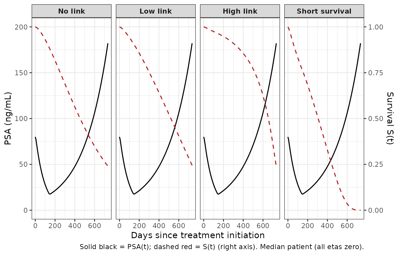
Replicates Figure 2 of Desmee 2015: median-patient PSA(t) (solid black) and survival S(t) (colored lines) for the four simulation scenarios. lambda and beta vary per scenario; all four use the same PSA-kinetic parameters.
End-of-study survival (calibration check)
The source paper states that lambda was calibrated per scenario so the median patient has approximately 25% survival at t = 735 days. We confirm:
end_sur <- trajectories |>
  group_by(scenario) |>
  filter(abs(time - 735) == min(abs(time - 735))) |>
  summarise(
    psa_t735  = round(psa, 2),
    cumhaz    = round(cumhaz, 4),
    sur_t735  = round(sur, 4),
    .groups = "drop"
  )

knitr::kable(
  end_sur,
  caption = "Median-patient PSA and survival at t = 735 days, by scenario. Compare sur_t735 to the paper's 25% calibration target (the 'Short survival' scenario was intentionally not held at 25%)."
)| scenario | psa_t735 | cumhaz | sur_t735 |
|---|---|---|---|
| No link | 182.14 | 1.4266 | 0.2401 |
| Low link | 182.14 | 1.4085 | 0.2445 |
| High link | 182.14 | 1.4451 | 0.2357 |
| Short survival | 182.14 | 10.3137 | 0.0000 |
For the three calibrated scenarios (No link, Low link, High link),
sur_t735 should be near 0.25. For “Short survival” (which
deliberately combines a high baseline hazard with a strong PSA link) the
median patient dies considerably earlier, so sur_t735 is
much lower.
Stochastic VPC at the population (subset, replicate Figure 3 spaghetti)
Figure 3 of the source paper shows spaghetti plots of N = 500 simulated PSA trajectories per scenario. We replicate the structure with a much smaller cohort (N = 60 per scenario) to keep the vignette under the pkgdown wall-clock budget.
n_sub <- 60L

make_cohort <- function(n, scenario_id_offset) {
  tibble::tibble(
    id = scenario_id_offset + seq_len(n)
  )
}

ev_obs <- rxode2::et(seq(0, 735, by = 21))   # PSA every 3 weeks

vpc <- scenarios |>
  rowwise() |>
  do({
    sc <- .
    offset <- 1000L * which(scenarios$scenario == sc$scenario)
    cohort <- make_cohort(n_sub, scenario_id_offset = offset)
    ev_cohort <- ev_obs |>
      rxode2::etExpand()
    s <- rxode2::rxSolve(
      mod, ev_obs,
      nSub = n_sub,
      params = c(llam_haz = log(sc$lambda),
                 e_psa_haz = sc$beta),
      returnType = "data.frame"
    )
    s$scenario <- sc$scenario
    s
  }) |>
  ungroup() |>
  mutate(scenario = factor(scenario, levels = scenarios$scenario))
#> intdy -- t = 588 illegal. t not in interval tcur - _rxC(hu) to tcur
#> intdy -- t = 609 illegal. t not in interval tcur - _rxC(hu) to tcur
#> intdy -- t = 630 illegal. t not in interval tcur - _rxC(hu) to tcur
#> intdy -- t = 651 illegal. t not in interval tcur - _rxC(hu) to tcur
#> intdy -- t = 672 illegal. t not in interval tcur - _rxC(hu) to tcur
#> intdy -- t = 693 illegal. t not in interval tcur - _rxC(hu) to tcur
#> intdy -- t = 714 illegal. t not in interval tcur - _rxC(hu) to tcur
#> intdy -- t = 735 illegal. t not in interval tcur - _rxC(hu) to tcur
#> intdy -- t = 714 illegal. t not in interval tcur - _rxC(hu) to tcur
#> intdy -- t = 735 illegal. t not in interval tcur - _rxC(hu) to tcur
#> intdy -- t = 714 illegal. t not in interval tcur - _rxC(hu) to tcur
#> intdy -- t = 735 illegal. t not in interval tcur - _rxC(hu) to tcur
#> intdy -- t = 735 illegal. t not in interval tcur - _rxC(hu) to tcur
#> intdy -- t = 567 illegal. t not in interval tcur - _rxC(hu) to tcur
#> intdy -- t = 588 illegal. t not in interval tcur - _rxC(hu) to tcur
#> intdy -- t = 609 illegal. t not in interval tcur - _rxC(hu) to tcur
#> intdy -- t = 630 illegal. t not in interval tcur - _rxC(hu) to tcur
#> intdy -- t = 651 illegal. t not in interval tcur - _rxC(hu) to tcur
#> intdy -- t = 672 illegal. t not in interval tcur - _rxC(hu) to tcur
#> intdy -- t = 693 illegal. t not in interval tcur - _rxC(hu) to tcur
#> intdy -- t = 714 illegal. t not in interval tcur - _rxC(hu) to tcur
#> intdy -- t = 735 illegal. t not in interval tcur - _rxC(hu) to tcur

vpc_median <- vpc |>
  group_by(scenario, time) |>
  summarise(psa_med = stats::median(psa), .groups = "drop")

vpc_typical <- trajectories |>
  select(scenario, time, psa) |>
  rename(psa_typ = psa)

ggplot(vpc, aes(time, psa, group = sim.id)) +
  geom_line(alpha = 0.15, linewidth = 0.25) +
  geom_line(
    data = vpc_median, aes(time, psa_med, group = NULL),
    color = "steelblue", linewidth = 0.9
  ) +
  geom_line(
    data = vpc_typical, aes(time, psa_typ, group = NULL),
    color = "darkorange", linewidth = 0.7, linetype = "dashed"
  ) +
  facet_wrap(~scenario, nrow = 2) +
  scale_y_log10() +
  labs(
    x = "Days since treatment initiation",
    y = "PSA (ng/mL, log scale)",
    caption = "Black = individual subjects; blue = empirical median across the 60-subject cohort; dashed orange = median patient (zero etas)."
  ) +
  theme_bw()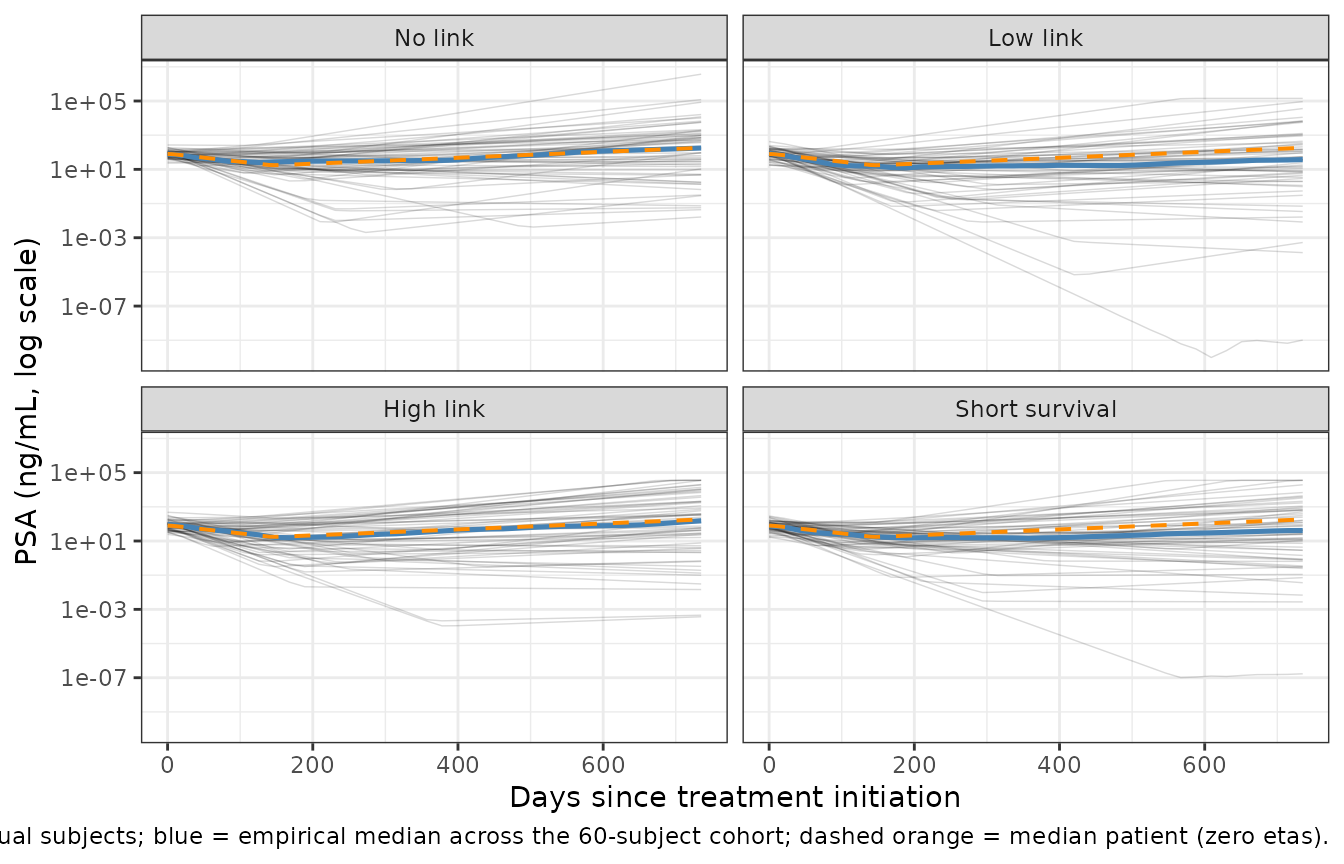
PSA spaghetti plots for 60 simulated subjects per scenario. Black thin lines = individual trajectories; thick blue line = empirical median; orange dashed = median patient (zero etas). Mirrors the per-scenario panels of Desmee 2015 Figure 3.
Quantitative summary of the stochastic cohorts
vpc_summary <- vpc |>
  group_by(scenario) |>
  summarise(
    median_psa_t0    = stats::median(psa[time == 0]),
    median_psa_tesc  = stats::median(psa[abs(time - 147) <= 11]),
    median_psa_t735  = stats::median(psa[abs(time - 735) <= 11]),
    median_sur_t735  = stats::median(sur[abs(time - 735) <= 11]),
    .groups = "drop"
  )

knitr::kable(
  vpc_summary,
  digits = 3,
  caption = "Stochastic-cohort summaries: median PSA at t=0 (should be near 80), near treatment escape (t~147 day), and at end-of-study (t=735 day); median survival probability at t=735."
)| scenario | median_psa_t0 | median_psa_tesc | median_psa_t735 | median_sur_t735 |
|---|---|---|---|---|
| No link | 78.849 | 27.418 | 176.883 | 0.240 |
| Low link | 85.682 | 15.684 | 37.312 | 0.349 |
| High link | 93.232 | 16.194 | 152.216 | 0.369 |
| Short survival | 75.881 | 17.565 | 41.389 | 0.060 |
The cohort medians should track the median-patient values from the preceding table to within Monte Carlo noise at N = 60.
Assumptions and deviations
-
High link scenario chosen as the canonical default.
The packaged model file fixes the survival parameters at the paper’s
“High link” values (
beta = 0.02,lambda = 2150,k = 1.5). The other three published scenarios are replicated in this vignette by passingparams =torxSolve, never by editing the model file. This matches the paper’s framing: PSA kinetics is one structural model, and the survival parameters are a per-scenario sensitivity dimension. -
PSA production rate
pset to 1. Eq. (3) of the source paper makes clear that the analytical PSA trajectory does not depend onp: at QSS,p * C(0) = delta * PSA0, andpcancels out of the PSA equation. The cell-count compartmentcellsis therefore in arbitrary “QSS units” and is not directly comparable to the source paper’s per-mL prostate-cell count. PSA(t) and the survival hazard are unaffected. - No covariates were retained from the source. The paper does not develop any covariate effects; all per-subject heterogeneity is encoded through the four etas.
-
Observation variable
logPSA1is not a canonical nlmixr2lib name.checkModelConventions()warns on this. The name reflects the paper’s log(PSA + 1) observation transform (Eq. 4) and is intentional; future registration oflogPSA<n>patterns in the conventions register would retire the warning. This is consistent with other paper-named PD outputs in the library (e.g.,tumor_volin the Cardilin 2018 and Simeoni 2004 oncology models). - Smaller stochastic cohort. The source paper simulated N = 500 per scenario; this vignette uses N = 60 per scenario to keep the pkgdown render under the 5-minute wall-clock budget. The qualitative spaghetti pattern and the median trajectories are unchanged.
-
A tiny epsilon
del_t = 1e-6is added inside the Weibull baseline hazard to keep the(t / lambda)^(k - 1)factor well-defined att = 0. Withk = 1.5 > 1the baseline hazard is zero att = 0regardless, so the epsilon does not change the integrated cumulative hazard. - No PKNCA validation. PKNCA is the wrong validation target for a biomarker-survival joint model with no PK structure; replication of the paper’s Figures 2 and 3 plus the end-of-study survival calibration check cover the corresponding ground.