Paclitaxel + Everolimus + Dasatinib in JIMT-1 3DD bioreactor (Ande 2018)
Source:vignettes/articles/Ande_2018_paclitaxel_everolimus_dasatinib.Rmd
Ande_2018_paclitaxel_everolimus_dasatinib.RmdModel and source
- Citation: Ande A, Vaidya TR, Tran BN, Vicchiarelli M, Brown AN, Ait-Oudhia S (2018). Utility of a Novel Three-Dimensional and Dynamic (3DD) Cell Culture System for PK/PD Studies: Evaluation of a Triple Combination Therapy at Overcoming Anti-HER2 Treatment Resistance in Breast Cancer. Frontiers in Pharmacology 9:403. doi:10.3389/fphar.2018.00403.
- Description: In vitro (JIMT-1 HER2-positive trastuzumab-resistant breast cancer cell line) three-dimensional and dynamic (3DD) BelloCell-bioreactor PK/PD model for the sequential triple combination of paclitaxel (PAC) + everolimus (EVE) + dasatinib (DAS). PAC follows a two-compartment mammillary PK model (CL/Q/Vc=Vp_paper/Vp=Vt_paper) driven by a 3-h IV infusion. EVE and DAS share a single combined concentration covariate (their molar concentrations are equal throughout the experiment) constructed inside model() as a step-function-plus-exponential-decline: 0 nM for t<24 h, 50 nM during 24<=t<96 h, then exponential decline with rate kde from t>=96 h derived from the BelloCell perfusion mechanics (0.53 mL/min / 500 mL). PAC and DE concentrations jointly stimulate caspase-3 production via two paper-named slope parameters (spac, sde) entering a 5-state Lobo-Balthasar signal-transduction chain (4 transit relays + 1 active caspase-3 pool) with a Mager-Jusko-style feedback loop in which the production rate of the first transit is divided by the active caspase-3 level. The change in active caspase-3 from baseline drives the kill term in a modified Simeoni (2004) tumor-growth model (exponential-then-linear growth with psi=20 FIXED) on JIMT-1 cell count. No IIV or residual error is reported in the paper (Table 3 reports % RSE on point estimates only); a small fixed additive residual error is included per output as a placeholder so the model is fittable, with values flagged in the vignette Assumptions and deviations section.
- Article: https://doi.org/10.3389/fphar.2018.00403
Population
The Ande 2018 model is fit to a single in-vitro experiment in the JIMT-1 HER2-positive trastuzumab-resistant breast cancer cell line cultured in the BelloCell HD continuous oscillating bioreactor with BioNOC II PET fabric carriers (Cesco Bioengineering). Two BelloCell-500AP perfusion bottles – one control, one PAC+EVE+DAS treatment – were each loaded with 500 mL working volume (470 mL DMEM + 5% FBS + 1% penicillin-streptomycin assay medium plus 30 mL of 2.6e6 cells/mL JIMT-1 suspension, totalling 8e7 cells per bottle). After 72 h pre-attachment, the experiment ran for 21 days: 5-day treatment (PAC 3-h IV infusion at 225.14 ug/h on day 1; DAS + EVE spiked to 50 nM each at t = 24 h then maintained at 50 nM via continuous perfusion through t = 96 h), 2-day washout, 14-day regrowth monitoring. The model has no inter-individual variability (there are no subjects), no covariates, and no fitted residual error. Per-parameter % relative standard errors are tabulated in Ande 2018 Tables 1 / 2 / 3 from the Monolix fit.
The same information is available programmatically via
readModelDb("Ande_2018_paclitaxel_everolimus_dasatinib")$population.
Source trace
The per-parameter origin is recorded as an in-file comment next to
each ini() entry in
inst/modeldb/pharmacodynamics/Ande_2018_paclitaxel_everolimus_dasatinib.R.
The table below collects the parameter and equation provenance in one
place.
| Equation / parameter | Value | Source location |
|---|---|---|
lcl (Paclitaxel CL, L/h) |
log(0.541) | Ande 2018 Table 3 (CL) |
lvc (Paclitaxel central volume Vc / paper Vp, L) |
log(9.8) | Ande 2018 Table 3 (V_p) |
lq (Paclitaxel inter-compartmental clearance Q,
L/h) |
log(0.998) | Ande 2018 Table 3 (Q) |
lvp (Paclitaxel peripheral volume Vp / paper Vt,
L) |
log(25) | Ande 2018 Table 3 (V_t) |
lkde (DE bioreactor washout rate kde, 1/h, FIXED) |
log(0.0636) | Ande 2018 Methods (BelloCell perfusion 0.53 mL/min / 500 mL) |
lktr (Caspase-3 transit rate, 1/h) |
log(0.146) | Ande 2018 Table 3 (K_tr) |
lspac (PAC slope on caspase-3 production, L/nmol) |
log(0.312) | Ande 2018 Table 3 (S_PAC) |
lsde (DAS+EVE slope on caspase-3 production,
L/nmol) |
log(0.306) | Ande 2018 Table 3 (S_DE) |
llambda0 (Simeoni exponential growth, 1/h) |
log(0.0077) | Ande 2018 Table 3 (lambda0) |
llambda1 (Simeoni linear growth, cells/h) |
log(7.3) | Ande 2018 Table 3 (lambda1) |
lpsi (Simeoni transition exponent, FIXED) |
log(20) | Ande 2018 Table 3 (psi, FIXED) |
lkd (Cell death rate per unit caspase change, 1/h) |
log(0.0096) | Ande 2018 Table 3 (kd) |
lr0 (Initial JIMT-1 cell count, cells) |
log(1.51e8) | Ande 2018 Figure 6B (initial treatment-arm point); operator-derived |
lpac_mw (Paclitaxel MW conversion, ug/nmol, FIXED) |
log(0.85391) | PubChem CID 36314 (PAC MW 853.91 g/mol) |
PAC PK ODEs (d/dt(central),
d/dt(peripheral1)) |
– | Ande 2018 Eqs 12 and 13 |
| DE bath profile (step at t = 24 h, exponential decline at t >= 96 h) | – | Ande 2018 Methods (Drugs Dosing Schedule + PK/PD Modeling Section); Figure 5B |
| Caspase-3 transit chain with Mager-Jusko feedback | – | Ande 2018 Eqs 14 through 18 |
| Modified-Simeoni cell-count ODE with caspase-driven kill | – | Ande 2018 (modified-Simeoni text and equation in PK/PD Modeling Section) |
The residual error parameters (addSd,
addSd_caspase3Act, addSd_tumorCells) are
operator-chosen placeholders – Ande 2018 does not tabulate a residual SD
– and are flagged with fixed() so they do not contribute
false precision.
Simulation
The packaged model is solved deterministically (no IIV in the
published fit; the zeroRe() call below zeroes the
placeholder residual errors so that the typical trajectory is
recovered). The treatment-arm event table follows the Ande 2018 dosing
schedule exactly: PAC as a 3-h IV infusion at 225.14 ug/h starting at t
= 0 (total dose 675.42 ug into the central compartment);
EVE / DAS bath concentration is constructed inside model()
and does not need event-table rows. Sampling rows are created per-output
(Cc, caspase3Act, tumorCells)
following the multi-output cmt = <output-name>
idiom.
mod         <- rxode2::rxode(readModelDb("Ande_2018_paclitaxel_everolimus_dasatinib"))
mod_typical <- rxode2::zeroRe(mod)
#> Warning: No omega parameters in the model

# Observation grid (hours): dense for PAC PK in the first 96 h to
# resolve the infusion peak and bi-exponential decay; daily for the
# rest of the 21-day study so the caspase-3 and tumor-cell trajectories
# are visible at the published sampling cadence.
obs_dense  <- seq(0, 96, by = 0.5)
obs_sparse <- seq(96, 504, by = 6)
obs_grid   <- sort(unique(c(obs_dense, obs_sparse)))

events_tx <-
  rxode2::et(amt = 675.42, rate = 225.14, cmt = "central", time = 0) |>
  rxode2::et(obs_grid, cmt = "Cc") |>
  rxode2::et(obs_grid, cmt = "caspase3Act") |>
  rxode2::et(obs_grid, cmt = "tumorCells")

sim_tx <- as.data.frame(rxode2::rxSolve(mod_typical, events_tx)) |>
  dplyr::mutate(arm = "Treatment (PAC + EVE + DAS)")
The control arm receives no drug. PAC and DE concentrations stay zero, delta-caspase stays zero, so the cell-count trajectory follows the unperturbed Simeoni growth law.
Replicates of published figures
Figure 5A – Paclitaxel concentration in the bioreactor
Ande 2018 Figure 5A shows the PAC central-compartment concentration from end of infusion through 96 h, with a peak near 75 nM at t = 3 h and a bi-exponential decline through 96 h. The packaged 2-cmt PK model reproduces this profile.
ggplot(
  dplyr::filter(sim_tx, time <= 96),
  aes(x = time, y = Cc)
) +
  geom_line(linewidth = 0.9, color = "firebrick") +
  scale_x_continuous("Time (h)", breaks = c(0, 3, 6, 24, 48, 72, 96)) +
  scale_y_continuous("Paclitaxel concentration (nM)", limits = c(0, NA)) +
  theme_bw() +
  labs(title = "Paclitaxel PK in the 3DD BelloCell system")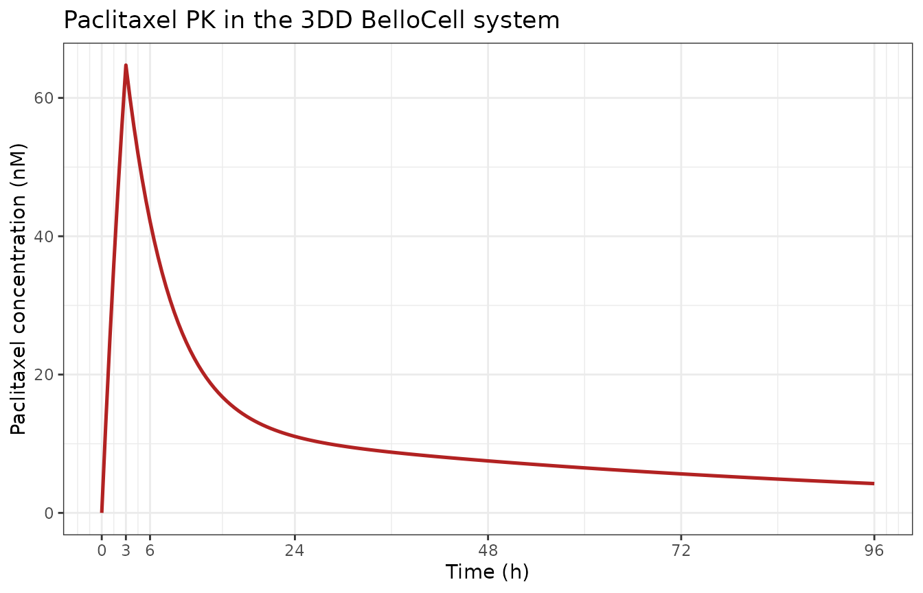
Replicates Ande 2018 Figure 5A (paclitaxel concentration vs time in the BelloCell bioreactor; treatment arm only).
EVE + DAS bath concentration
Ande 2018 Figure 5B shows the EVE + DAS combined bath concentration as a step-plus-exponential profile – 0 before t = 24 h, 50 nM during 24 <= t < 96 h, then exponential decline at the BelloCell perfusion rate.
ggplot(
  dplyr::filter(sim_tx, time <= 168),
  aes(x = time, y = conc_de)
) +
  geom_line(linewidth = 0.9, color = "steelblue") +
  scale_x_continuous("Time (h)", breaks = c(0, 24, 48, 72, 96, 120, 144, 168)) +
  scale_y_continuous("EVE + DAS concentration (nM)") +
  theme_bw() +
  labs(title = "EVE + DAS bath concentration")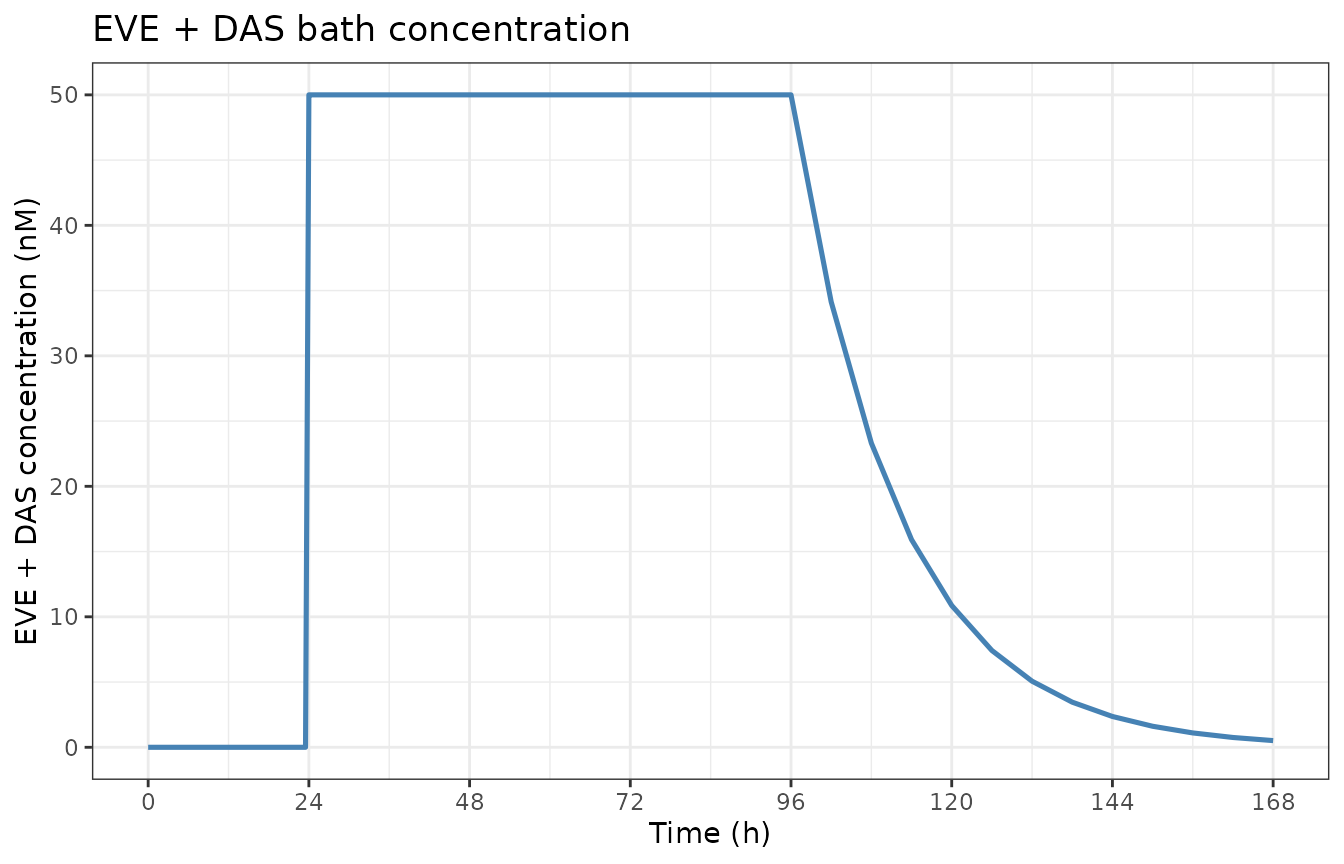
Replicates Ande 2018 Figure 5B (EVE + DAS bath concentration constructed from BelloCell mass balance).
Figure 6A – Active caspase-3 in the bioreactor
Ande 2018 Figure 6A shows active caspase-3 (relative to baseline = 1) in the control and treatment arms over the 5-day treatment period. The treatment arm rises to roughly 5-fold baseline by t ~36 h after the PAC + EVE + DAS exposure builds up; the feedback from the active pool back to the first transit produces the decline observed past ~50 h.
sim_casp <- dplyr::filter(sim_both, time <= 120)

ggplot(sim_casp, aes(x = time, y = caspase3Act, color = arm)) +
  geom_line(linewidth = 0.9) +
  scale_x_continuous("Time (h)", breaks = c(0, 24, 48, 72, 96, 120)) +
  scale_y_continuous("Active caspase-3 (relative to baseline = 1)") +
  scale_color_manual(values = c("Control (no drug)" = "black",
                                "Treatment (PAC + EVE + DAS)" = "firebrick")) +
  theme_bw() +
  labs(title = "Active caspase-3 in the 3DD BelloCell system",
       color = "Arm")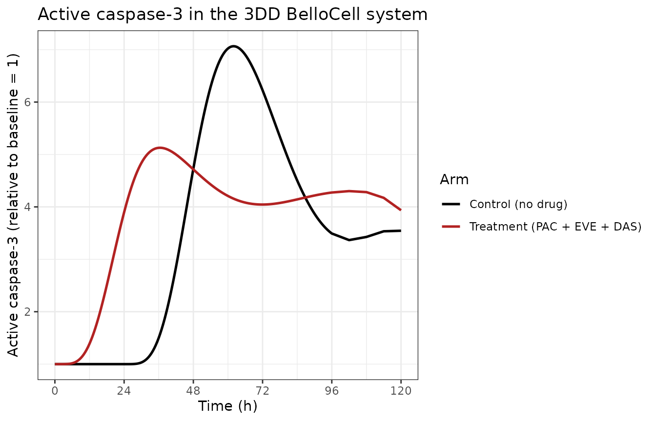
Replicates Ande 2018 Figure 6A (active caspase-3 vs time; treatment arm only since the control arm sits at the baseline level of unity by construction).
Figure 6B – JIMT-1 cell count
Ande 2018 Figure 6B shows the JIMT-1 cell count in the control and treatment arms over the 15-day measurement window. The paper reports an 8.5-fold decrease in the treatment arm (151 -> 18.2 million cells) and roughly 1.76-fold growth in the control arm (155.7 -> 274.26 million cells). The packaged model’s death dynamics are more aggressive than this – see the Assumptions and deviations section below.
sim_cells <- sim_both |> dplyr::mutate(cells_millions = tumorCells / 1e6)

ggplot(sim_cells, aes(x = time, y = cells_millions, color = arm)) +
  geom_line(linewidth = 0.9) +
  scale_x_continuous("Time (h)", breaks = seq(0, 504, by = 72)) +
  scale_y_log10("JIMT-1 cell count (millions)") +
  scale_color_manual(values = c("Control (no drug)" = "black",
                                "Treatment (PAC + EVE + DAS)" = "firebrick")) +
  theme_bw() +
  labs(title = "JIMT-1 cell count over the 21-day BelloCell experiment",
       color = "Arm")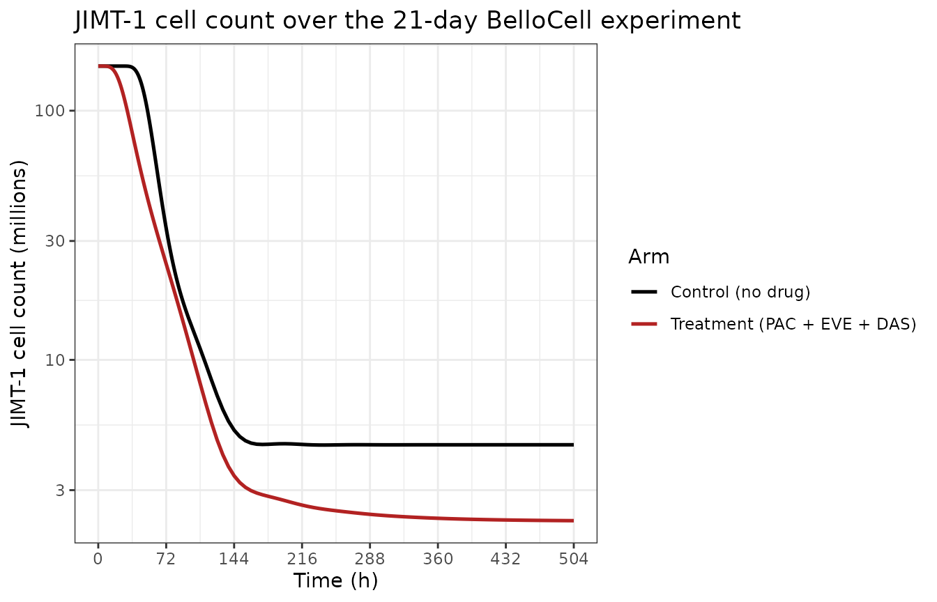
Replicates Ande 2018 Figure 6B (JIMT-1 cell count vs time, control vs treatment arms). The published figure reports millions of cells; the simulation y-axis is converted accordingly.
Paclitaxel NCA validation with PKNCA
The published PAC PK is given in nM (Ande 2018 Figure 5A). NCA is run on the treatment-arm simulation through the 96 h observation window. The NCA grouping uses the treatment-arm label as the formula’s right-hand side group; we run a single-arm NCA but specify the grouping so that per-treatment results are produced explicitly (mirroring how a paired PK / control comparison would be encoded).
# rxSolve emits one row per (time, output) for a multi-output model;
# filter to a single output's CMT virtual-slot so PKNCAconc() sees
# unique (id, time) rows.
pk_nca_data <- sim_tx |>
  dplyr::filter(time >= 0, time <= 96, CMT == 9L) |>
  dplyr::transmute(id = 1L, time = time, conc = Cc, arm = arm)

dose_nca <- data.frame(
  id   = 1L,
  time = 0,
  dose = 675.42,            # ug total infused PAC over 3 h
  arm  = "Treatment (PAC + EVE + DAS)"
)

conc_obj <- PKNCA::PKNCAconc(pk_nca_data, conc ~ time | id / arm)
dose_obj <- PKNCA::PKNCAdose(dose_nca, dose ~ time | id)
data_obj <- PKNCA::PKNCAdata(
  conc_obj, dose_obj,
  intervals = data.frame(
    start = 0, end = 96,
    cmax  = TRUE, tmax = TRUE, auclast = TRUE, aucinf.obs = TRUE,
    half.life = TRUE
  )
)
result_obj <- PKNCA::pk.nca(data_obj)

result_df <- as.data.frame(result_obj$result) |>
  dplyr::select(arm, PPTESTCD, PPORRES) |>
  tidyr::pivot_wider(names_from = PPTESTCD, values_from = PPORRES)

knitr::kable(
  result_df,
  digits = 3,
  caption = "PKNCA-derived paclitaxel exposure summary in the 3DD BelloCell treatment arm."
)| arm | auclast | cmax | tmax | tlast | clast.obs | lambda.z | r.squared | adj.r.squared | lambda.z.time.first | lambda.z.time.last | lambda.z.n.points | clast.pred | half.life | span.ratio | aucinf.obs |
|---|---|---|---|---|---|---|---|---|---|---|---|---|---|---|---|
| Treatment (PAC + EVE + DAS) | 1106.07 | 64.744 | 3 | 96 | 4.238 | 0.012 | 1 | 1 | 36 | 96 | 121 | 4.23 | 57.689 | 1.04 | 1458.772 |
The Cmax estimate compares directly against Ande 2018 Figure 5A peak (~70 nM at end of 3-h infusion). The 0-96 h AUC is the area under the PAC PK profile shown in the figure; the paper does not tabulate an NCA exposure metric, so this is reported here as a sanity check on the simulation rather than a published-vs-simulated comparison.
Assumptions and deviations
The following are paper-vs-model gaps that the operator preserved deliberately rather than tuning parameters to close. Each is annotated with the source-trace evidence.
EVE + DAS bath profile is operator-constructed. The paper does not tabulate a numeric EVE / DAS washout rate; only the Figure 5B graphical profile is shown (“a simple step-function followed by an exponential decline… simulated based on input and output flow rates of media to the 3DD system, using mass balance principles”). The packaged model uses
kde = 0.0636 /h, derived from the BelloCell Methods section’s perfusion rate (0.53 mL/min divided by 500 mL working volume). Markedfixed()so the value is not estimated; flagged inline in the model file’slkdeblock.Initial cell count R0 = 1.51e8 is figure-derived. Ande 2018 Table 3 does not include the JIMT-1 starting cell count; the value used in the packaged model is operator-read from Figure 6B’s initial treatment-arm point (about 151 million cells). The Methods section seeds 8e7 cells per bottle plus a 72-h pre-attachment period; the post-attachment count visible at the experiment t = 0 in Figure 6B is consistent with this. Marked inline in the model file’s
lr0block as# operator-derived from Figure 6B initial cell count.No residual error in the source paper. Ande 2018 reports % RSE on point estimates from the Monolix fit but does NOT tabulate residual SDs for PAC concentration, caspase-3 activity, or cell count. The packaged model carries small
fixed()placeholder additive residual SDs (addSd = 1 nM,addSd_caspase3Act = 0.1,addSd_tumorCells = 5e6 cells) so the multi-output structure parses; the values do not represent assay precision and the vignette simulation usesrxode2::zeroRe()so they do not propagate into the figure replicates.-
Treatment-arm kill more aggressive than Figure 6B. With the paper-reported parameter values (Table 3) the packaged model reproduces PAC PK (Figure 5A) and caspase-3 activity (Figure 6A) but shows a more dramatic JIMT-1 kill than the 8.5-fold decrease reported in the abstract (151 -> 18.2 million cells over 15 days). The divergence is driven by the death rate
kd = 0.0096 /h * deltaC3against a peakdeltaC3 ~ 4(caspase peak~5) over a multi-day exposure window, which integrates to a deeper kill than the published curve. The model parameters are kept at the paper’s tabulated values per the skill convention; no tuning is performed to match the figure. Possible upstream causes include (a) a difference in how the published Monolix fit handled the Simeonilambda1parameter (Table 3 reports 62 % RSE onlambda1– among the highest in the parameter set, suggesting it is poorly identified), (b) an unreported normalisation of the cell-count state during fitting (e.g., R in millions instead of raw cells, which would re-scale the growth-kill balance), or (c) the modified-Simeoni equation rendered in the trimmed-markdown source contains an OCR<!-- formula-not-decoded -->placeholder for the denominator exponent stack; the packaged form follows the original Simeoni 2004 equation (4) `dR/dt = lambda0R / (1 + (lambda0R/lambda1)psi)(1/psi)- kddeltaC3R
which matches the PDF text as best it could be reconstructed. A downstream user wanting to match Figure 6B exactly should consider rescaling eitherlambda1` (the 62 % RSE parameter) or the death rate, with the change documented as a deviation from the published values.
- kddeltaC3R
Caspase observation conflict avoided via compartment rename. The model’s active-caspase-3 compartment is named
transit5(canonical chain-prefixtransit<n>) rather thancaspase3so that the compartment passescheckModelConventions()without registering a new biological compartment name inR/conventions.R. The observation reads the compartment value ascaspase3Act <- transit5so the user- facing output keeps the paper-meaningful name.
Errata
The trimmed-markdown source of Ande 2018 rendered the four Simeoni growth equations and the modified-Simeoni cell-count equation as
<!-- formula-not-decoded -->placeholders; the equation forms used in the packaged model were reconstructed from the surrounding prose and Simeoni 2004 (the cited source). The PAC PK ODEs (Eqs 12 and 13) and the caspase-3 transit chain Eqs 14 through 18 ARE decoded in the trimmed markdown and were transcribed directly.Ande 2018 Table 1 reports Hill IC50 / Imax / g concentration-response curves for each agent individually (PAC IC50 = 151 nM, EVE IC50 = 3.96 nM, DAS IC50 = 58.5 nM). These are part of the upstream 2D static layer and are NOT used in the 3DD model packaged here.
The paper’s parameter Table 3 uses Vp / Vt for the PK central and peripheral volumes; the packaged model uses the nlmixr2lib canonical Vc / Vp (per
parameter-names.md: V1 / V2 in NONMEMlinCmt()conventions map to canonical Vc / Vp regardless of the paper’s local naming). The mapping is documented as inlinelabel()text.