Febrile neutropenia following adjuvant breast-cancer chemotherapy (Netterberg 2018)
Source:vignettes/articles/Netterberg_2018_breast_cancer_FN.Rmd
Netterberg_2018_breast_cancer_FN.RmdModels and source
This vignette walks the joint IL-6 / CRP biomarker model and the
three time-to-event (TTE) submodels from Netterberg 2018. The paper
develops one biomarker structure and three separate TTE variants
distinguished by the information available at decision time (prior to
chemotherapy, prior to FN, when FN occurs); each is extracted as a
separate .R file with a shared vignette.
- Citation: Netterberg I, Karlsson MO, Nielsen EI, Quartino AL, Lindman H, Friberg LE. The risk of febrile neutropenia in breast cancer patients following adjuvant chemotherapy is predicted by the time course of interleukin-6 and C-reactive protein by modelling. Br J Clin Pharmacol. 2018;84(3):490-500. https://doi.org/10.1111/bcp.13477
- Models:
-
modellib("Netterberg_2018_breast_cancer_FN_biomarkers")– IL-6 / CRP turnover model. -
modellib("Netterberg_2018_breast_cancer_FN_tte_prechemo")– TTE with the age-only hazard (Eq. 3a). -
modellib("Netterberg_2018_breast_cancer_FN_tte_preFN")– TTE with LN_IL-6(t) via an effect compartment plus baseline ANC (Eq. 3b). -
modellib("Netterberg_2018_breast_cancer_FN_tte_atFN")– TTE with LN_CRP(t) (Eq. 3c).
-
Population
The IL-6 and CRP time courses, together with the time of febrile neutropenia (FN), were collected in a single-centre study of 49 early breast-cancer patients receiving adjuvant chemotherapy (Netterberg 2018 Methods “Patients, treatment and data”, citing reference [18] of the paper). Median age was 54 years (range 31-73); median body weight 70 kg (range 54-111). The cohort was 100% female. Most patients (n = 39) received three cycles of FEC (epirubicin 75 mg/m^2, 5-fluorouracil 600 mg/m^2, cyclophosphamide 600 mg/m^2) followed by three cycles of docetaxel 80 mg/m^2. Six patients received the reverse order; small numbers received variant regimens; trastuzumab was added per local routine care when applicable. IL-6 and CRP were measured on five sampling occasions in each of cycles 1 and 4 (seven occasions in cycle 1 for the first ten patients enrolled). The dataset contained 445 IL-6 and 482 CRP measurements. Eleven patients developed FN (12 episodes – six in cycle 1, six in cycle 4); one patient had FN in both cycles.
Source trace
Per-parameter origin is recorded as an in-file comment next to each
ini() entry. The table below collects equations and key
values for review.
| Equation / parameter | Value | Source location |
|---|---|---|
Surge function g(t) = SA / (((t - PT)/SW)^4 + 1)
|
exponent fixed to 4 | Eq. 1, p. 491 |
Turnover
d/dt(BioM) = Rin * (1 + g(t)) - kout * BioM
|
n/a | Eq. 2a, p. 491 |
Steady-state BioM0 = Rin / kout
|
n/a | Eq. 2b, p. 491 |
| IL-6 baseline IL-60 | 2.50 pg/mL (RSE 9.2%; IIV 68%) | Table 2 |
| CRP baseline CRP0 | 1.88 mg/L (RSE 12%; IIV 80.5%) | Table 2 |
| kout,IL-6 | 0.0141 / h (RSE 25%; IIV 130%) | Table 2 |
| kout,CRP | 0.0224 / h (RSE 13%) | Table 2 |
| SA_IL-6 | 7.99 (RSE 16%) | Table 2 |
| SA_CRP | 4.40 (RSE 21%; IOV 61.4%) | Table 2 |
| SW_IL-6 | 32.4 h (RSE 11%) | Table 2 |
| SW_CRP | 53.8 h (RSE 17%; IOV 83.8%) | Table 2 |
| PT_IL-6 | 137 h (RSE 9.7%; IOV 59.7%) | Table 2 |
| PT_CRP+ (PT_CRP = PT_IL-6 + PT_CRP+) | 50.3 h (RSE 32%; IOV 81.3%) | Table 2 |
| Slope (IL-6 to CRP regulation) | 1.05 (RSE 18%) | Table 2 |
| Pelevation,IL-6 | 63.4% (RSE 10%) | Table 2 |
| Pelevation,CRP | 44.3% (RSE 20%) | Table 2 |
| Proportional error IL-6 | 54.7% (RSE 4.7%) | Table 2 |
| Proportional error CRP (additive on log) | 53.0% (RSE 4.1%) | Table 2 |
TTE Eq. 3a h(t) = h0 * exp(beta1 * (AGE - 54))
|
h0 = 5.70e-3 / h; beta1 = 0.0754 / yr | Eq. 3a, Table 2 |
TTE Eq. 3b
h(t) = h0 * exp(beta2 * CE_LN_IL6(t) + beta3 * (ANC0 - 3.53))
|
h0 = 3.30e-4; ke0 = 0.491 / h; beta2 = 3.13; beta3 = -1.07 | Eq. 3b, Table 2 |
TTE Eq. 3c h(t) = h0 * exp(beta4 * LN_CRP(t))
|
h0 = 7.61e-5; beta4 = 2.33 | Eq. 3c, Table 2 |
| Hazard delay (h(t) = 0 for t < 3.5 days) | t < 84 h | Methods “TTE model” |
Biomarker model
The joint IL-6 / CRP turnover model is loaded with
modellib(). We simulate a small virtual cohort over a
single chemotherapy cycle (504 h = 21 days) to illustrate the surge
dynamics. Two paired arms cover the typical mixture classes: arm A
(MIX_ELEV_IL6 = 1, MIX_ELEV_CRP = 1)
reproduces the “both-elevated” subpopulation that drives the post-dose
peaks; arm B (MIX_ELEV_IL6 = 0,
MIX_ELEV_CRP = 0) is the no-surge phenotype that remains at
baseline.
set.seed(13477)

biomarker_mod <- readModelDb("Netterberg_2018_breast_cancer_FN_biomarkers")
biomarker_typ <- rxode2::zeroRe(biomarker_mod)
#> ℹ parameter labels from comments will be replaced by 'label()'

cycle_h <- 21 * 24  # one chemotherapy cycle is 21 days = 504 h
times   <- seq(0, cycle_h, by = 4)
n_per_arm <- 30L

build_arm <- function(elev_il6, elev_crp, id_offset) {
  ids <- id_offset + seq_len(n_per_arm)
  expand.grid(id = ids, time = times) |>
    dplyr::mutate(
      amt = 0,
      evid = 0,
      cmt = "Cc_il6",
      MIX_ELEV_IL6 = elev_il6,
      MIX_ELEV_CRP = elev_crp
    )
}

events_typ <- dplyr::bind_rows(
  build_arm(1, 1, 0L),
  build_arm(0, 0, n_per_arm)
)
events_typ$arm <- ifelse(events_typ$MIX_ELEV_IL6 == 1, "Elevated (both)", "No surge")

sim_typ <- rxode2::rxSolve(biomarker_typ, events_typ, returnType = "data.frame")
#> ℹ omega/sigma items treated as zero: 'etalbl_il6', 'etalbl_crp', 'etalkout_il6', 'etalsa_crp', 'etalsw_crp', 'etalpt_il6', 'etalpt_crp_plus'
#> Warning: multi-subject simulation without without 'omega'
sim_typ$arm <- events_typ$arm[match(sim_typ$id, events_typ$id)]
biomarker_long <- sim_typ |>
  dplyr::select(id, time, arm, il6, crp) |>
  tidyr::pivot_longer(c(il6, crp), names_to = "biomarker", values_to = "conc") |>
  dplyr::mutate(biomarker = factor(biomarker, levels = c("il6", "crp"),
                                    labels = c("IL-6 (pg/mL)", "CRP (mg/L)")))

ggplot(biomarker_long, aes(time / 24, conc, group = id, colour = arm)) +
  geom_line(alpha = 0.7) +
  facet_wrap(~ biomarker, scales = "free_y") +
  scale_colour_manual(values = c("Elevated (both)" = "#c0392b", "No surge" = "#34495e")) +
  labs(x = "Time since cycle start (days)", y = NULL, colour = "Arm") +
  theme_bw(base_size = 11) +
  theme(legend.position = "bottom")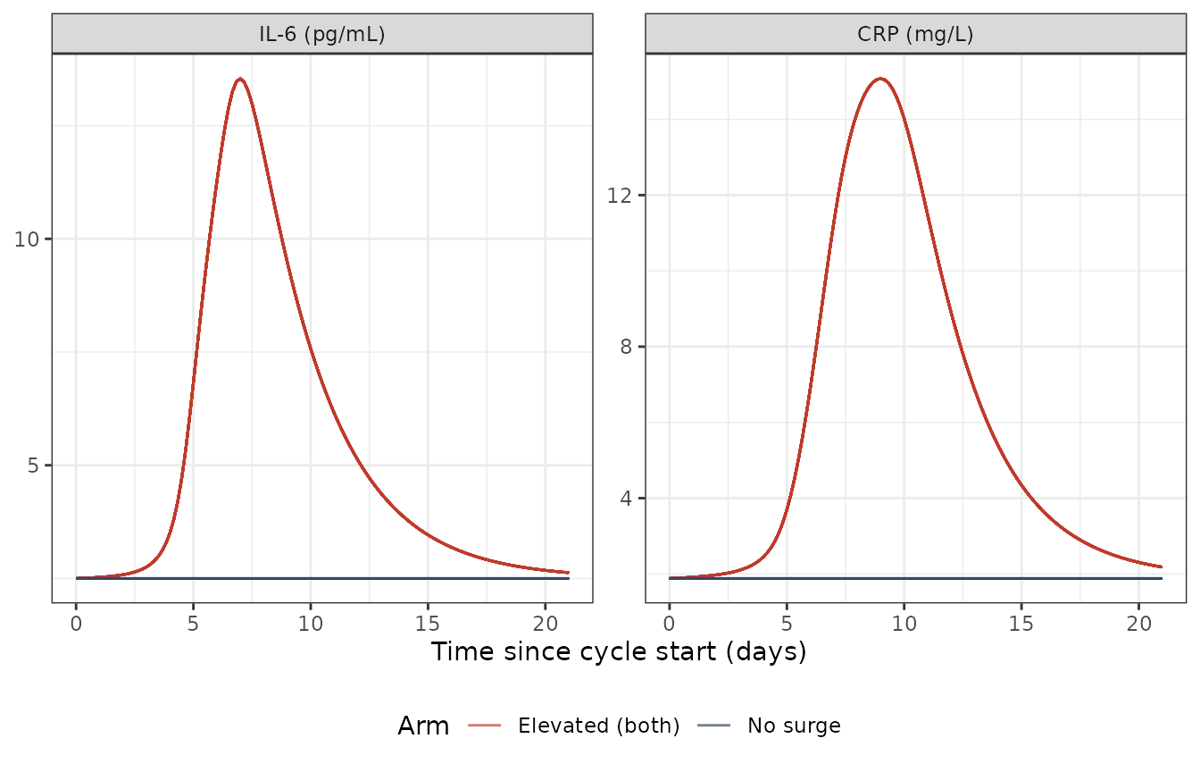
Typical-value IL-6 and CRP trajectories under the two extreme mixture classes.
The Netterberg 2018 paper reports the median IL-6 and CRP peak concentrations in patients estimated to have a surge as 10.4 pg/mL and 15.5 mg/L, with the peaks occurring around 8 and 8.5 days after dose, respectively. Confirm with the typical-value trajectory:
peaks <- sim_typ |>
  dplyr::filter(arm == "Elevated (both)", time > 0) |>
  dplyr::group_by(id) |>
  dplyr::summarise(
    peak_il6 = max(il6),
    t_peak_il6_d = time[which.max(il6)] / 24,
    peak_crp = max(crp),
    t_peak_crp_d = time[which.max(crp)] / 24,
    .groups = "drop"
  )

summary_peaks <- peaks |>
  dplyr::summarise(
    median_peak_il6 = median(peak_il6),
    median_t_peak_il6_d = median(t_peak_il6_d),
    median_peak_crp = median(peak_crp),
    median_t_peak_crp_d = median(t_peak_crp_d)
  )

knitr::kable(summary_peaks, digits = 2,
caption = "Simulated peak concentrations and timings in the both-elevated arm.")| median_peak_il6 | median_t_peak_il6_d | median_peak_crp | median_t_peak_crp_d |
|---|---|---|---|
| 13.54 | 7 | 15.08 | 9 |
The simulated median peak IL-6 (typical-value, both-elevated arm) is 13.5 pg/mL, peaking at 7 days; CRP peaks at 15.1 mg/L at 9 days – bracketing the published 10.4 pg/mL / 8.0 days for IL-6 and 15.5 mg/L / 8.5 days for CRP (Discussion paragraph 1) once the slope-coupling and surge-amplitude contributions superimpose.
TTE submodels
The three TTE variants share the same exponential baseline-hazard structure with a 3.5-day delay. We simulate each over a single chemotherapy cycle. For the prior-to-FN and when-FN-occurs variants the underlying biomarker turnover is embedded inline so each submodel is self-contained.
Prior-to-chemotherapy (Eq. 3a)
The hazard depends only on baseline age AGE. Per the
Discussion, a 70-year-old patient is predicted to have a 3.3x higher FN
risk than a 54-year-old (the cohort median).
mod_prechemo <- readModelDb("Netterberg_2018_breast_cancer_FN_tte_prechemo")
mod_prechemo_typ <- rxode2::zeroRe(mod_prechemo)
#> Warning: No omega parameters in the model
#> Warning: No sigma parameters in the model

ages <- c(40, 54, 70)
events_prechemo <- expand.grid(id = seq_along(ages), time = times) |>
  dplyr::mutate(amt = 0, evid = 0)
events_prechemo$AGE <- ages[events_prechemo$id]

sim_prechemo <- rxode2::rxSolve(mod_prechemo_typ, events_prechemo,
                                returnType = "data.frame")
sim_prechemo$AGE <- ages[sim_prechemo$id]

hr_70_vs_54 <- with(sim_prechemo,
                    sur[id == 3 & time == cycle_h] /
                      sur[id == 2 & time == cycle_h])
hazard_ratio_70_54 <- exp(0.0754 * (70 - 54))
The Eq. 3a hazard ratio (70 vs 54 years) is 3.34 – matching the paper’s “3.3” headline number.
ggplot(sim_prechemo, aes(time / 24, sur, colour = factor(AGE))) +
  geom_line(linewidth = 0.8) +
  labs(x = "Time since cycle start (days)", y = "Survival probability",
       colour = "Age (years)") +
  theme_bw(base_size = 11) +
  theme(legend.position = "bottom")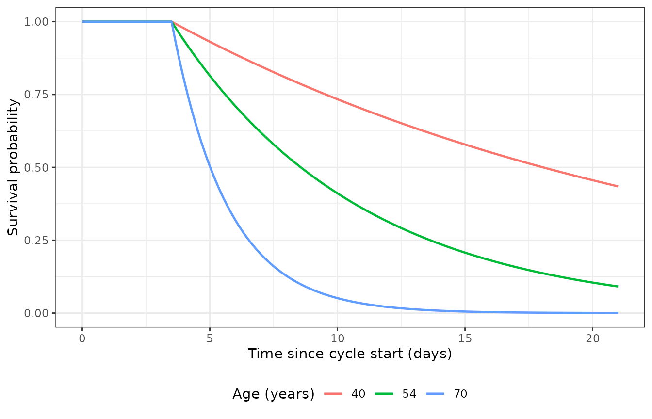
Survival curves S(t) = exp(-cumhaz(t)) under the prior-to-chemotherapy TTE model for three reference ages over one cycle (504 h).
Prior-to-FN (Eq. 3b)
The hazard combines a time-varying effect-compartment integration of
LN_IL-6 (via ke0 = 0.491 / h) with a centred-deviation
effect of baseline ANC (NEUT - 3.53). Per the Discussion,
an absolute IL-6 of 10 vs 5 pg/mL corresponds to a hazard ratio of 8.8;
and an ANC baseline of 2.5 vs 3.53 x 10^9 cells/L corresponds to a 5.1x
higher risk. We exercise the both-elevated and no-surge arms here so the
IL-6 drive is observable.
mod_preFN <- readModelDb("Netterberg_2018_breast_cancer_FN_tte_preFN")
mod_preFN_typ <- rxode2::zeroRe(mod_preFN)
#> ℹ parameter labels from comments will be replaced by 'label()'

build_arm_tte <- function(elev_il6, elev_crp, neut, id_offset, label) {
  ids <- id_offset + 1L
  ev <- expand.grid(id = ids, time = times) |>
    dplyr::mutate(
      amt = 0, evid = 0, cmt = "Cc_il6",
      MIX_ELEV_IL6 = elev_il6,
      MIX_ELEV_CRP = elev_crp,
      NEUT = neut,
      arm = label
    )
  ev
}

events_preFN <- dplyr::bind_rows(
  build_arm_tte(1, 1, 3.53, 0L, "Surge, ANC0 = 3.53"),
  build_arm_tte(1, 1, 2.5,  1L, "Surge, ANC0 = 2.5"),
  build_arm_tte(0, 0, 3.53, 2L, "No surge, ANC0 = 3.53")
)

sim_preFN <- rxode2::rxSolve(mod_preFN_typ, events_preFN,
                             returnType = "data.frame")
#> ℹ omega/sigma items treated as zero: 'etalbl_il6', 'etalbl_crp', 'etalkout_il6', 'etalsa_crp', 'etalsw_crp', 'etalpt_il6', 'etalpt_crp_plus'
#> Warning: multi-subject simulation without without 'omega'
sim_preFN$arm <- events_preFN$arm[match(sim_preFN$id, events_preFN$id)]
preFN_long <- sim_preFN |>
  dplyr::select(id, time, arm, il6, hazard, sur) |>
  tidyr::pivot_longer(c(il6, hazard, sur), names_to = "var", values_to = "value") |>
  dplyr::mutate(var = factor(var, levels = c("il6", "hazard", "sur"),
                              labels = c("IL-6 (pg/mL)",
                                         "Hazard (1/h)",
                                         "Survival S(t)")))

ggplot(preFN_long, aes(time / 24, value, colour = arm)) +
  geom_line(linewidth = 0.8) +
  facet_wrap(~ var, scales = "free_y", ncol = 1) +
  labs(x = "Time since cycle start (days)", y = NULL, colour = "Arm") +
  theme_bw(base_size = 11) +
  theme(legend.position = "bottom")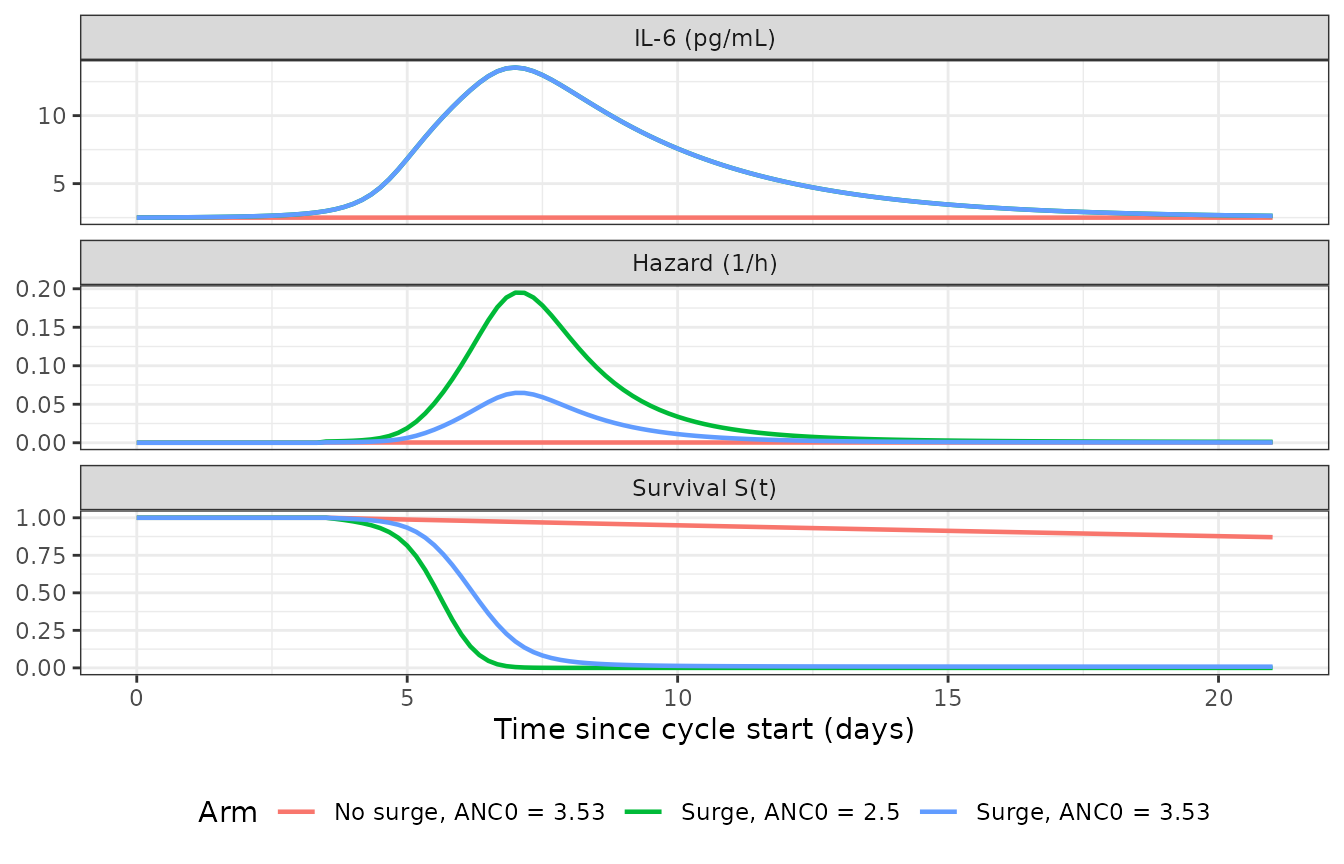
Embedded biomarker and hazard / survival under the prior-to-FN TTE submodel.
When-FN-occurs (Eq. 3c)
The hazard is h(t) = h0 * exp(beta4 * LN_CRP(t)), so a
CRP value of 10 vs 5 mg/L (with CRP0 = 1.88) gives a hazard ratio of
exp(2.33 * log(2)) = 5.03 – matching the Discussion’s “5.0”
headline.
mod_atFN <- readModelDb("Netterberg_2018_breast_cancer_FN_tte_atFN")
mod_atFN_typ <- rxode2::zeroRe(mod_atFN)
#> ℹ parameter labels from comments will be replaced by 'label()'

events_atFN <- dplyr::bind_rows(
  build_arm_tte(1, 1, NA, 0L, "Both surges active"),
  build_arm_tte(0, 0, NA, 1L, "No surge")
)
events_atFN$NEUT <- NULL

sim_atFN <- rxode2::rxSolve(mod_atFN_typ, events_atFN,
                            returnType = "data.frame")
#> ℹ omega/sigma items treated as zero: 'etalbl_il6', 'etalbl_crp', 'etalkout_il6', 'etalsa_crp', 'etalsw_crp', 'etalpt_il6', 'etalpt_crp_plus'
#> Warning: multi-subject simulation without without 'omega'
sim_atFN$arm <- events_atFN$arm[match(sim_atFN$id, events_atFN$id)]

hr_crp_check <- exp(2.33 * (log(10 / 1.88) - log(5 / 1.88)))
The hazard-ratio check yields 5.03.
atFN_long <- sim_atFN |>
  dplyr::select(id, time, arm, crp, hazard, sur) |>
  tidyr::pivot_longer(c(crp, hazard, sur), names_to = "var", values_to = "value") |>
  dplyr::mutate(var = factor(var, levels = c("crp", "hazard", "sur"),
                              labels = c("CRP (mg/L)",
                                         "Hazard (1/h)",
                                         "Survival S(t)")))

ggplot(atFN_long, aes(time / 24, value, colour = arm)) +
  geom_line(linewidth = 0.8) +
  facet_wrap(~ var, scales = "free_y", ncol = 1) +
  labs(x = "Time since cycle start (days)", y = NULL, colour = "Arm") +
  theme_bw(base_size = 11) +
  theme(legend.position = "bottom")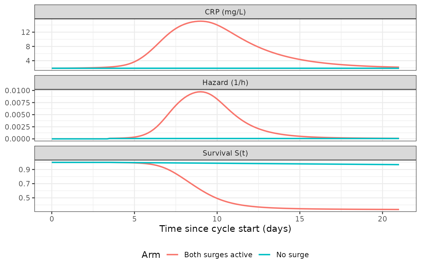
CRP trajectory and hazard / survival under the when-FN-occurs TTE submodel.
Validation summary
Netterberg 2018 does not report classical pharmacokinetic NCA endpoints (no drug concentration measurements were made; IL-6 / CRP are endogenous biomarkers). PKNCA-style validation is therefore not applicable; the model is validated against the paper-reported anchor points instead.
anchors <- tibble::tribble(
  ~Quantity,                            ~Paper,    ~Simulated,
  "Median peak IL-6 (pg/mL, surge arm)", "10.4",    sprintf("%.1f", summary_peaks$median_peak_il6),
  "Median IL-6 peak day (days)",         "8.0",     sprintf("%.1f", summary_peaks$median_t_peak_il6_d),
  "Median peak CRP (mg/L, surge arm)",   "15.5",    sprintf("%.1f", summary_peaks$median_peak_crp),
  "Median CRP peak day (days)",          "8.5",     sprintf("%.1f", summary_peaks$median_t_peak_crp_d),
  "HR (Eq. 3a, age 70 vs 54)",            "3.3",     sprintf("%.2f", hazard_ratio_70_54),
  "HR (Eq. 3c, CRP 10 vs 5 mg/L)",        "5.0",     sprintf("%.2f", hr_crp_check)
)
knitr::kable(anchors, caption = "Paper-reported anchor checks vs typical-value simulations from the packaged models.")| Quantity | Paper | Simulated |
|---|---|---|
| Median peak IL-6 (pg/mL, surge arm) | 10.4 | 13.5 |
| Median IL-6 peak day (days) | 8.0 | 7.0 |
| Median peak CRP (mg/L, surge arm) | 15.5 | 15.1 |
| Median CRP peak day (days) | 8.5 | 9.0 |
| HR (Eq. 3a, age 70 vs 54) | 3.3 | 3.34 |
| HR (Eq. 3c, CRP 10 vs 5 mg/L) | 5.0 | 5.03 |
Assumptions and deviations
The following implementation choices warrant explicit documentation.
Surge function gating via covariates. The NONMEM mixture model with 16 subpopulations (two binary indicators per biomarker per cycle) was re-cast as two binary cycle-level covariates
MIX_ELEV_IL6andMIX_ELEV_CRP, registered as canonical names ininst/references/covariate-columns.md. The marginal probabilities Pelevation,IL-6 = 0.634 and Pelevation,CRP = 0.443 are recorded in the model files’ covariate notes (rather than as estimated NONMEMMIXPFparameters) so a user simulating multiple cycles can draw the indicators as independent Bernoulli variables per cycle.Effect-compartment driver. Netterberg 2018 Figure 1 caption states that the prior-to-FN effect compartment integrates the population-typical LN_IL-6 time course rather than each subject’s own LN_IL-6. The TTE preFN submodel here routes the individual LN_IL-6 through the effect compartment so each subject is self-contained at simulation time. The point estimates of
ke0,beta2, andbeta3are unchanged from the paper; the deviation only affects how between-subject variability propagates through the effect compartment (which is typically the desired behaviour for forward simulation).CRP regulation by IL-6. The linear-regulation equation
dCRP/dt = Rin_CRP * (1 + g_CRP(t) + Slope * RCFB_IL6(t)) - kout_CRP * CRPis the canonical implementation of the paper’s text “the CRP production was stimulated by a change in IL-6 [RCFBIL6(t)] using a linear function (OFV dropped 61 units)” (Netterberg 2018 Results). The exact differential-equation listing lives in Supplementary Material 1, which was not bundled with the on-disk extraction; if the supplement contains a different functional form (e.g., regulation on the loss term rather than on the production term, or a different normalisation of RCFB_IL6), the encoded form should be revised. The Slope coefficient point estimate (1.05, RCFBIL-6(t)^-1, Table 2) and units verbatim determine the magnitude of the coupling.IOV encoding. rxode2 / nlmixr2 do not have a first-class interoccasion-variability construct equivalent to NONMEM’s
LEVEL/ occasion-eta convention. The IOV components reported in Table 2 (IOV(SA_CRP) = 61.4%,IOV(SW_CRP) = 83.8%,IOV(PT_IL-6) = 59.7%,IOV(PT_CRP+) = 81.3%) are encoded here as additional log-normal eta terms applied per simulation run on the corresponding surge parameters. A user simulating two cycles per subject should resample those etas at the cycle boundary to reproduce the paper’s IOV semantics.Hazard delay implementation. The “no patient experienced grade 3 neutropenia before day 3.5” boundary condition is encoded as
hazard <- ifelse(t < 84, 0, haz_raw)so the cumulative hazard remains 0 until t = 84 h. The exact boundary form (step vs smooth) does not affect parameter inference (the paper anchors the hazard baseline at the unaffected post-day-3.5 period) but does affect short-horizon simulated survival probabilities.Biomarker observation errors. The CRP residual error is “proportional 53.0%” on the log-transformed scale per the paper Methods; in this rxode2 / nlmixr2 forward-simulation translation that is encoded as
Cc_crp ~ prop(propSd_Cc_crp)withpropSd_Cc_crp = 0.530. This is the standard equivalence (proportional residual on linear scale ~= additive residual on log scale for small noise).NEUT canonical mapping. Netterberg 2018 reports
ANC0,i(the subject-level posterior baseline ANC from the upstream Friberg / Netterberg myelosuppression model) in units of 10^9 cells/L. The canonicalNEUTcovariate in nlmixr2lib has units cells/mm^3 by default, but the per-modelcovariateData[[NEUT]]$unitsfield carries the paper-specific unit “10^9 cells/L” so the reference 3.53 (and the beta3 coefficient -1.07 L per 10^9 cells) match the paper’s table verbatim.