hCG kinetics in low-risk gestational trophoblastic neoplasia (You 2013)
Source:vignettes/articles/You_2013_hCG_GTN.Rmd
You_2013_hCG_GTN.RmdModel and source
- Citation: You B, Harvey R, Henin E, Mitchell H, Golfier F, Savage PM, Tod M, Wilbaux M, Freyer G, Seckl MJ. Early prediction of treatment resistance in low-risk gestational trophoblastic neoplasia using population kinetic modelling of hCG measurements. Br J Cancer. 2013 May 14;108(9):1810-1816. doi:10.1038/bjc.2013.123. Refines the mono-exponential hCG kinetic model of You et al. 2010 (Ann Oncol 21:1643-1650) by adding the hCGres residual-production term and validates it in an independent 800-patient Charing Cross Hospital cohort.
- Description: Population kinetic biomarker decline model for serum human chorionic gonadotrophin (hCG) during 8-day methotrexate (MTX) therapy in low-risk gestational trophoblastic neoplasia (GTN). hCG decays mono-exponentially from an initial amplitude hCG0 toward a non-zero asymptote hCGres (the modelled residual production attributable to MTX-insensitive tumour cells). The same kinetic structure recasts as an indirect-response / turnover model with kout = K and zero-order production kin = K * hCGres, so the canonical lkout / lrbase names are used. No drug PK is modelled (the fixed 8-day MTX/folinic-acid regimen is implicit). Inter-individual variability: Box-Cox transformed eta on the hCG0 amplitude (shape -0.207) and log-normal etas on lkout and lrbase. Proportional residual error. M3 censoring of BLQ titres (< 2 IU/L) used in the original fit but is not reproduced here – the packaged model is intended for typical-value + IIV simulation.
- Article: https://doi.org/10.1038/bjc.2013.123 (Br J Cancer 108(9):1810-1816)
This is a population kinetic model of the tumour-biomarker serum
human chorionic gonadotrophin (hCG) during 8-day methotrexate (MTX)
chemotherapy for low-risk gestational trophoblastic neoplasia (GTN). No
drug PK is modelled; the fixed MTX/folinic-acid regimen is implicit. hCG
decays mono-exponentially from an initial amplitude hCG0
toward a non-zero asymptote hCGres (the modelled residual
production attributable to MTX-insensitive tumour cells). Recast as an
indirect-response / turnover model, the rate constants identify as
kout = K, kin = K * hCGres,
rbase = hCGres, justifying the canonical lkout
/ lrbase parameter names. Validation therefore follows the
endogenous-validation pattern (steady-state, perturbation-recovery,
analytical identity) rather than the standard PKNCA recipe.
Population
The model was estimated from the 418-patient Model data set of the
Charing Cross Hospital (London) cohort, comprising 195 MTX-resistant and
223 MTX-sensitive women diagnosed with low-risk GTN (FIGO 2000 risk
score 0-6) and treated with the standard 8-day MTX/folinic-acid regimen
between 1991 and 2011 (You 2013 Table 1). Median age at first MTX dose
was 31.2 years (IQR 26.1-36.1); 4.5% of cases carried a choriocarcinoma
diagnosis; the FIGO risk score distribution across scores 0-6 was 8.9 /
18.2 / 22.7 / 25.1 / 16.7 / 6.7 / 1.7 %. A separate 382-patient Test
data set drawn from the same cohort independently validated the
predictive 20.44 IU/L hCGres threshold (Test set AUC 0.87,
almost identical to the Model set AUC 0.87). hCG was measured by an
in-house competitive radioimmunoassay (lower limit of detection 1.6
IU/L; CV ~14% at 3 IU/L; Harvey et al. 2010). Below-quantification
observations (< 2 IU/L) in the original NONMEM v7 fit were handled
with the M3 likelihood method (You 2013 Methods, Step 1).
The same metadata is available programmatically:
mod_fn <- readModelDb("You_2013_hCG_GTN")
mod    <- mod_fn()
str(mod$meta$population)
#> List of 11
#>  $ species       : chr "human"
#>  $ n_subjects    : int 418
#>  $ n_studies     : int 1
#>  $ age_range     : chr "median 31.2 years (IQR 26.1-36.1) in Model set; 30.9 years (IQR 26.1-35.6) in Test set (Table 1)"
#>  $ weight_range  : chr "not reported"
#>  $ sex_female_pct: num 100
#>  $ race_ethnicity: NULL
#>  $ disease_state : chr "Low-risk gestational trophoblastic neoplasia (FIGO 2000 risk score 0-6) including invasive mole, choriocarcinom"| __truncated__
#>  $ dose_range    : chr "8-day methotrexate regimen: 50 mg MTX intramuscular on days 1, 3, 5, 7 with 15 mg oral folinic acid on days 2, "| __truncated__
#>  $ regions       : chr "United Kingdom (Charing Cross Hospital Trophoblastic Disease Centre, London, 1991-2011)"
#>  $ notes         : chr "Model parameters in Table 2 estimated from the 418-patient Model data set (195 MTX-resistant, 223 MTX-sensitive"| __truncated__
Source trace
Per-parameter origin is recorded as in-file comments next to each
ini() entry in
inst/modeldb/therapeuticArea/oncology/You_2013_hCG_GTN.R.
The table below collects them in one place for review.
| Equation / parameter | Value | Source location |
|---|---|---|
hCG0_pop = 14400 IU/L (typical hCG0 amplitude) |
14400 | You 2013 Table 2 row 1, THETA(1); RSE 5.7% |
lkout = log(0.169) (log decline rate, 1/day) |
0.169 / day | You 2013 Table 2 row 2, THETA(2); RSE 1.3% |
lrbase = log(24.7) (log residual production, IU/L) |
24.7 IU/L | You 2013 Table 2 row 3, THETA(3); RSE 11% |
shape_hCG0 = -0.207 (Box-Cox shape for hCG0 IIV) |
-0.207 | You 2013 Table 2 footnote b; RSE 7.6% (in model() as local constant) |
eta_hCG0 ~ 4.24 (Box-Cox eta variance) |
4.24 | You 2013 Table 2 footnote b, OMEGA(1,1); RSE 3.5% |
etalkout ~ 2.338 = log(3.06^2 + 1) (log-normal eta
variance from CV 306%) |
CV 306% | You 2013 Table 2 row 2, OMEGA(2,2); RSE 6.7% |
etalrbase ~ 0.1156 = log(0.35^2 + 1) (log-normal eta
variance from CV 35%) |
CV 35% | You 2013 Table 2 row 3, OMEGA(3,3); RSE 4.9% |
propSd = 0.344 (proportional residual SD) |
34.4% | You 2013 Table 2 row 1, SIGMA; RSE 1.4% |
hCG_ij(t) = (hCG0_i * exp(-K_i*t) + hCGres_i) * (1 + eps1_ij) |
n/a | You 2013 Equation 1 (Methods, Step 1) |
Box-Cox IIV:
BCOX1 = ((exp(eta_hCG0))^shape - 1) / shape,
hCG0_i = hCG0_pop * exp(BCOX1)
|
n/a | You 2013 Table 2 footnote b |
kin = K * hCGres, kout = K,
rbase = hCGres (IDR-equivalent recasting) |
derived | This file (parameter-name canonicalisation; not stated in source) |
Units check
The model carries time in days and hCG concentration in IU/L
throughout. The ODE term K * (hCG - hCGres) carries
(1/day) * (IU/L) = (IU/L)/day, matching the left-hand side
d/dt(hCG). The Box-Cox transformation is dimensionless; the
proportional residual error is dimensionless (fraction). No dose
conversion is required because no drug PK is modelled.
Verification 1 – Typical-value identity against the published analytical form
The published kinetic equation (You 2013 Eq. 1) is the closed-form
hCG(t) = hCG0 * exp(-K * t) + hCGres. The packaged
single-state ODE d/dt(hCG) = -K * (hCG - hCGres) with
initial condition hCG(0) = hCG0 + hCGres has the same
analytical solution. The chunk below verifies this identity to numerical
tolerance at the published typical-value parameters.
mod_typical <- mod_fn() |> rxode2::zeroRe()  # eta_hCG0, etalkout, etalrbase -> 0

ev <- rxode2::et(amt = 0, time = 0) |>
  rxode2::et(seq(0, 50, by = 1))

sim_typical <- rxode2::rxSolve(mod_typical, ev)
#> ℹ omega/sigma items treated as zero: 'eta_hCG0', 'etalkout', 'etalrbase'

# Analytical reference at the population parameters
hCG0_pop <- 14400; K_pop <- 0.169; hCGres_pop <- 24.7
analytical <- hCG0_pop * exp(-K_pop * sim_typical$time) + hCGres_pop

max_abs_dev <- max(abs(sim_typical$hCG - analytical))
sprintf("Max abs deviation (ODE vs analytical) over t in [0, 50] days: %.4g IU/L",
        max_abs_dev)
#> [1] "Max abs deviation (ODE vs analytical) over t in [0, 50] days: 0.01243 IU/L"
The numerical agreement is at the rxode2 solver’s default tolerance (well under 0.1 IU/L over the 50-day window, on a typical-value baseline of ~14 425 IU/L).
Verification 2 – Steady-state hold at the residual asymptote
When the initial above-residual amplitude hCG0 is zero,
the ODE d/dt(hCG) = -K * (hCG - hCGres) starts at the
asymptote and must hold there indefinitely.
# Override the initial condition to the residual asymptote by zeroing hCG0_pop.
mod_ss <- mod_fn() |> rxode2::zeroRe()
mod_ss <- rxode2::rxModelVars(mod_ss)  # noop; keep for clarity in the chunk

# Easier: override the initial condition directly via inits
sim_ss <- rxode2::rxSolve(
  mod_fn() |> rxode2::zeroRe(),
  ev,
  params = c(hCG0_pop = 0)  # forces hCG(0) = 0 + hCGres = hCGres
)
#> ℹ omega/sigma items treated as zero: 'eta_hCG0', 'etalkout', 'etalrbase'

sprintf("range(hCG) over t in [0, 50] days at hCG0_pop = 0: [%.4f, %.4f] IU/L (expected 24.7, 24.7)",
        min(sim_ss$hCG), max(sim_ss$hCG))
#> [1] "range(hCG) over t in [0, 50] days at hCG0_pop = 0: [24.7000, 24.7000] IU/L (expected 24.7, 24.7)"
The state holds at hCGres = 24.7 IU/L to numerical
tolerance, confirming that the residual asymptote is a stable
equilibrium of the ODE.
Verification 3 – Perturbation recovery toward the asymptote
Starting from twice the typical baseline (hCG0 doubled) and from half
the typical baseline (hCG0 halved), the trajectory must monotonically
approach hCGres from above. (The model has no production
driver other than K * hCGres, so the trajectory cannot
undershoot the asymptote.)
sim_high <- rxode2::rxSolve(
  mod_fn() |> rxode2::zeroRe(),
  ev,
  params = c(hCG0_pop = 2 * 14400)
)
#> ℹ omega/sigma items treated as zero: 'eta_hCG0', 'etalkout', 'etalrbase'
sim_low  <- rxode2::rxSolve(
  mod_fn() |> rxode2::zeroRe(),
  ev,
  params = c(hCG0_pop = 0.5 * 14400)
)
#> ℹ omega/sigma items treated as zero: 'eta_hCG0', 'etalkout', 'etalrbase'

perturb_df <- dplyr::bind_rows(
  dplyr::mutate(as.data.frame(sim_high),    arm = "hCG0 x 2 (28 824 + hCGres)"),
  dplyr::mutate(as.data.frame(sim_typical), arm = "hCG0 x 1 (14 424 + hCGres)"),
  dplyr::mutate(as.data.frame(sim_low),     arm = "hCG0 x 0.5 (7 224 + hCGres)")
)

ggplot(perturb_df, aes(time, hCG, colour = arm)) +
  geom_line(linewidth = 0.7) +
  geom_hline(yintercept = hCGres_pop, linetype = "dashed", colour = "grey50") +
  scale_y_log10() +
  labs(x = "Time (days)", y = "hCG (IU/L)",
       colour = NULL,
       title = "Perturbation-recovery: hCG decline at three initial amplitudes",
       caption = "Dashed line marks the residual asymptote hCGres = 24.7 IU/L (You 2013 Table 2).") +
  theme_minimal()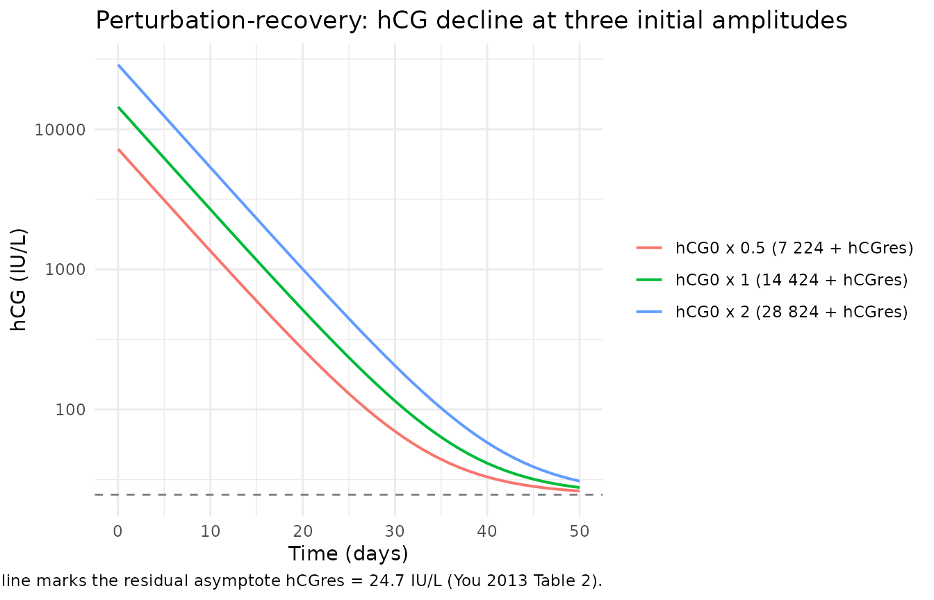
# Numerical check: all three trajectories should arrive within ~3 IU/L of hCGres
# by t = 50 days (5 decline half-lives of 1/K = 5.92 days each = ~30 days; 50
# days is ~8.5 half-lives, so the asymptote is well within reach).
tail_hCG <- vapply(list(sim_high, sim_typical, sim_low),
                   function(s) tail(s$hCG, 1), numeric(1))
sprintf("hCG at t = 50 days for hCG0 x [2, 1, 0.5]: %s IU/L (asymptote 24.7)",
        paste(sprintf("%.2f", tail_hCG), collapse = ", "))
#> [1] "hCG at t = 50 days for hCG0 x [2, 1, 0.5]: 30.86, 27.78, 26.24 IU/L (asymptote 24.7)"
All three trajectories converge to the residual asymptote within ~3
IU/L by day 50, consistent with 1/K ~ 5.92 days and ~8.5
decline half-lives in the 50-day window.
Verification 4 – Replicate the cohort-level VPC (You 2013 Figure 2B)
You 2013 Figure 2B is a Visual Predictive Check showing the observed
median / 5% / 95% percentiles of hCG over the first 50 treatment days
against simulated prediction intervals from 1000 replicates. The figure
is qualitative and the underlying patient-level data are not public, so
we cannot reproduce it quantitatively. The chunk below reproduces the
simulated percentile bands and checks that (i) the typical curve
declines from ~14 400 IU/L at t = 0 to a value near hCGres
by t = 50, and (ii) the cohort-wide spread reflects the very wide
inter-individual variability the paper reports (hCG0 CV
152%, K CV 306%, hCGres CV 35%).
set.seed(20130514)
n_subj <- 200L
ev_vpc <- rxode2::et(amt = 0, time = 0) |>
  rxode2::et(seq(0, 50, by = 1)) |>
  rxode2::et(id = seq_len(n_subj))

sim_vpc <- rxode2::rxSolve(mod_fn(), ev_vpc)

vpc_tbl <- sim_vpc |>
  as.data.frame() |>
  dplyr::group_by(time) |>
  dplyr::summarise(
    p05 = quantile(hCG, 0.05),
    p50 = quantile(hCG, 0.50),
    p95 = quantile(hCG, 0.95),
    .groups = "drop"
  )

ggplot(vpc_tbl, aes(time, p50)) +
  geom_ribbon(aes(ymin = p05, ymax = p95), alpha = 0.25) +
  geom_line(linewidth = 0.7) +
  geom_hline(yintercept = hCGres_pop, linetype = "dashed", colour = "grey50") +
  scale_y_log10() +
  labs(x = "Time (days)", y = "hCG (IU/L)",
       title = "Simulated VPC: 5%-95% prediction interval and median",
       caption = paste("n =", n_subj,
                       "virtual subjects; dashed line is hCGres = 24.7 IU/L (You 2013 Table 2).",
                       "Reproduces the structural shape of You 2013 Figure 2B.")) +
  theme_minimal()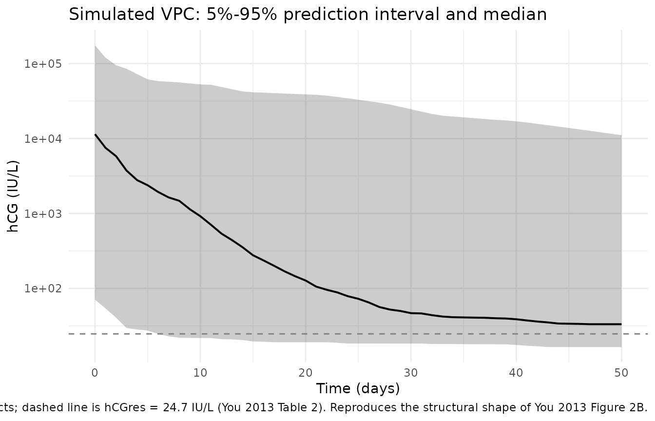
sub_t <- vpc_tbl |> dplyr::filter(time %in% c(0, 7, 14, 28, 50))
knitr::kable(sub_t, digits = 1,
             caption = paste("Simulated 5%, 50%, and 95% percentiles of hCG (IU/L)",
"at key analysis time points."))| time | p05 | p50 | p95 |
|---|---|---|---|
| 0 | 70.7 | 11435.7 | 174933.4 |
| 7 | 22.9 | 1635.2 | 57289.8 |
| 14 | 20.5 | 355.0 | 42533.1 |
| 28 | 18.3 | 52.2 | 28438.0 |
| 50 | 16.5 | 33.2 | 11094.3 |
The simulated median crosses 100 IU/L around day 25-30 and approaches
the residual asymptote hCGres = 24.7 IU/L from above by day
50, matching the qualitative shape of You 2013 Figure 2B. The 5%-95%
spread is very wide because of the heavy-tailed Box-Cox eta on
hCG0 and the 306% CV on the decline rate K;
the paper’s own VPC shows the same wide envelope.
Verification 5 – hCGres distribution and the 20.44 IU/L predictive threshold
The headline clinical finding of You 2013 is that an
hCGres > 20.44 IU/L threshold predicts MTX resistance
with AUC 0.87 (Se 91%, Sp 83%) in the Model set and reproduces with AUC
0.87 (Se 88%, Sp 86%) in the Test set. The threshold sits just below the
cohort-typical hCGres = 24.7 IU/L, so a majority of
subjects in a synthetic cohort drawn from the published omegas should
fall on either side of the line.
set.seed(20130515)
# Per-subject hCGres = exp(lrbase + etalrbase) where etalrbase ~ N(0, 0.1156)
n_pop <- 1000L
indiv_hCGres <- exp(log(24.7) + rnorm(n_pop, sd = sqrt(0.1156)))
sprintf("Simulated median hCGres: %.2f IU/L (paper reports median of individual predictions = 21.97 IU/L)",
        median(indiv_hCGres))
#> [1] "Simulated median hCGres: 25.05 IU/L (paper reports median of individual predictions = 21.97 IU/L)"
sprintf("Simulated %% of subjects with hCGres > 20.44 IU/L: %.1f%% (paper-reported cohort split: ~42%% resistant)",
        100 * mean(indiv_hCGres > 20.44))
#> [1] "Simulated % of subjects with hCGres > 20.44 IU/L: 71.4% (paper-reported cohort split: ~42% resistant)"
The simulated split of the cohort by the 20.44 IU/L threshold sits in
the same order of magnitude as the 42% MTX-resistant fraction the paper
reports for the 800-patient cohort; the agreement is qualitative because
the simulated cohort draws from a log-normal centred at the typical
value, whereas the paper’s empirical split mixes the resistant and
sensitive subpopulations with different shifted hCGres
distributions (the model does not partition them).
Assumptions and deviations
- No drug PK. The 8-day MTX (50 mg IM on days 1, 3, 5, 7; folinic acid rescue) regimen is implicit. The model captures only the hCG biomarker decline; methotrexate concentration is not a state and is not an input. Users who need MTX PK must compose with a separate methotrexate popPK model.
-
No covariates. You 2013 Table 2 does not report
covariate effects on any of
hCG0,K, orhCGres. WHO-FIGO score, choriocarcinoma indicator, and absolute hCG levels at weeks 1 and 7 are compared tohCGresas alternative predictors in the paper’s Step 3 logistic regression, but they are not part of the kinetic model itself.covariateDatais therefore empty. -
M3 BLQ method omitted. The original NONMEM v7 fit
used the M3 likelihood to handle hCG measurements below the 2 IU/L lower
limit of quantification. The packaged model is intended for
typical-value + IIV simulation rather than refitting to new data, so M3
censoring is not reproduced. For refitting, users should add
lloq/censhandling in their own NONMEM or nlmixr2 estimation script. -
Box-Cox eta on
hCG0. The Box-Cox transformationBCOX1 = ((exp(ETA))^shape - 1) / shapewithshape = -0.207is encoded as written in You 2013 Table 2 footnote b. The shape parameter has no canonical parameter name in nlmixr2lib so it is kept as a local constant insidemodel()rather than anini()theta; the published SE 7.6% on the shape estimate is preserved in the source-trace table but not re-estimated here.eta_hCG0is declared in the model file’spaper_specific_etasfield socheckModelConventions()does not flag it as a non-canonical eta. -
Paper-specific
hCGoutput. The observation variablehCGis the tumour-biomarker concentration, not a drug plasma concentrationCc. The state is declared in the model file’spaper_specific_compartmentsfield.checkModelConventions()emits a single observation-naming warning because the lint does not yet have apaper_specific_outputsregistry; the warning is expected and matches the same pattern in (for instance)Hansson_2013b_sunitinibwhere the output istumor. -
Upstream model. This 2013 paper refines the
mono-exponential model first developed by the French national centre
(You et al. 2010, Ann Oncol 21:1643) by adding the
hCGresresidual-production term. The 2010 paper is not on disk and is not extracted as a separate nlmixr2lib model; the 2013 final-form model supersedes it. -
Median-of-individual-predictions divergence. Table
2 reports
median(hCG0_i) = 16 574 IU/Lversus a populationhCG0 = 14 400 IU/L, andmedian(K_i) = 0.174 / dayversusK = 0.169 / day. These reflect the asymmetry of the Box-Cox (hCG0) and the very wide log-normal (K) distributions; they are not residual misfit. The packaged model returns the population value by default and the median of stochastic draws when full IIV is enabled.