Coproporphyrin I (Yoshida 2018, rifampin)
Source:vignettes/articles/Yoshida_2018_coproporphyrin_I_rifampin.Rmd
Yoshida_2018_coproporphyrin_I_rifampin.RmdModel and source
- Citation: Yoshida K, Guo C, Sane R. Quantitative Prediction of OATP-Mediated Drug-Drug Interactions With Model-Based Analysis of Endogenous Biomarker Kinetics. CPT Pharmacometrics Syst. Pharmacol. 2018;7(8):517-524. doi:10.1002/psp4.12315. The rifampin-CPI calibration (Table 2 left column) was fit to the Lai et al. 2016 plasma CPI profile cohort using portal-vein rifampin concentrations from the Simcyp v16r1 default single-dose rifampin model file as the forcing function; that Simcyp output is not reproducible from on-disk sources, so users must supply CP_RIF_UM externally. The companion GDC-0810 calibration is parameterised in modellib(‘Yoshida_2018_coproporphyrin_I_GDC0810’).
- Description: One-compartment endogenous turnover model for the OATP1B-substrate biomarker coproporphyrin I (CPI) in healthy adults (Yoshida 2018, rifampin-CPI calibration). CPI is produced at a zero-order synthesis rate Ksyn = kdeg * Baseline and eliminated as a single first-order pool whose overall rate constant kdeg is decomposed into a non-hepatic fraction fNH (unaffected by inhibitor) and a hepatic fraction 1 - fNH (competitively inhibited by the OATP1B perpetrator via Ki,u). The perpetrator portal-vein unbound concentration enters as a time-varying covariate CP_RIF_UM (umol/L); setting CP_RIF_UM = 0 collapses the model to the inhibitor-free steady state Baseline. This file encodes the rifampin-CPI calibration (Table 2 left column; no IIV reported); a sibling file Yoshida_2018_coproporphyrin_I_GDC0810 encodes the GDC-0810 calibration with its own Ki,u, kdeg, and IIV structure. The original fit used a Simcyp v16r1 default single-dose rifampin model for the portal-vein concentration profile; that PBPK output is not reproducible from on-disk sources and the paper itself documents an approximately 5-fold sensitivity of the estimated Ki,u to the choice of perpetrator-PK model, so downstream users must supply CP_RIF_UM externally and treat the calibrated Ki,u as conditional on that choice.
- Article: https://doi.org/10.1002/psp4.12315
Population and biological context
Coproporphyrin I (CPI) is a heme-biosynthesis byproduct and a
selective endogenous substrate of the hepatic OATP1B1 / OATP1B3
transporters. Yoshida 2018 proposed a simple one-compartment turnover
model for plasma CPI in which the overall first-order degradation rate
constant kdeg is split into a non-hepatic fraction
fNH (unaffected by perpetrator) and a hepatic fraction
1 - fNH that is competitively inhibited by the OATP1B
perpetrator via the unbound inhibition constant Ki,u. The
synthesis rate is anchored to the steady-state identity
Ksyn = kdeg * Baseline, so when the perpetrator
concentration is zero the model returns to the baseline CPI plasma
level.
This file encodes the rifampin-CPI calibration (Table 2 left column). The underlying clinical dataset is the Lai et al. 2016 cohort (12 healthy male SLCO1B1 c.521 T>C wildtype subjects); a single 600 mg oral dose of rifampin was used as the OATP1B perpetrator and Simcyp-predicted portal-vein unbound rifampin concentrations drove the inhibition term during fitting. The Yoshida 2018 fit did not estimate IIV for this analysis.
The same context is available programmatically via
readModelDb("Yoshida_2018_coproporphyrin_I_rifampin")$population.
Source trace
| Equation / parameter | Value | Source location |
|---|---|---|
lrbase |
log(0.863) | Yoshida 2018 Table 2, RIF-CPI column ‘Baseline (nM)’ = 0.863 (RSE 4.61%) |
lkdeg |
log(2.55) | Yoshida 2018 Table 2, RIF-CPI column ‘kdeg (1/h)’ = 2.55 (RSE 8.88%) |
logitfnh |
qlogis(0.129) | Yoshida 2018 Table 2, RIF-CPI column ‘fNH’ = 12.9 % (RSE 6.66%); estimated |
lkiu |
log(0.0203) | Yoshida 2018 Table 2, RIF-CPI column ‘Ki,u (uM)’ = 0.0203 (RSE 17.0%) |
propSd |
0.0513 | Yoshida 2018 Table 2, RIF-CPI column ‘Proportional residual error’ = 5.13 %CV |
| ODE form | n/a | Yoshida 2018 Methods (Model-based analysis with inhibitor kinetics) and Figure S1b |
| Steady-state baseline (analytic) | Ksyn / kdeg = Baseline |
Derived from d(Cc)/dt = 0 with no inhibitor:
Cc_ss = Baseline = 0.863 nmol/L
|
Units of every ODE term (dimensional analysis)
The Yoshida 2018 parameterisation operates directly on the plasma CPI
concentration (there is no explicit volume of distribution). The state
variable central carries the same units as Cc
(nmol/L); ksyn and the elimination flux therefore both have
units of nmol/L/h.
Term in d/dt(central) = ksyn - kdeg_eff * central
|
Units |
|---|---|
central (state) and Cc
|
nmol/L |
kdeg and kdeg_eff
|
1/h |
ksyn = kdeg * rbase |
nmol/L/h |
kdeg_eff * central |
nmol/L/h |
d/dt(central) |
nmol/L/h ok |
Steady-state check (no rifampin, deterministic typical-value)
With CP_RIF_UM = 0 the inhibition term collapses to
kdeg_eff = kdeg and the analytic steady-state plasma CPI is
Baseline = 0.863 nmol/L. The simulator should hold this
value indefinitely.
mod <- readModelDb("Yoshida_2018_coproporphyrin_I_rifampin")
mod_typical <- rxode2::zeroRe(mod)
#> Warning: No omega parameters in the model

make_cpi_events <- function(t_end = 200, dt = 2, crif = 0) {
  data.frame(
    id   = 1L,
    time = seq(0, t_end, by = dt),
    evid = 0L,
    amt  = 0,
    cmt  = "Cc",
    CP_RIF_UM = crif
  )
}

ss_sim <- rxode2::rxSolve(mod_typical, events = make_cpi_events(t_end = 200))
cat("Yoshida 2018 (RIF-CPI) typical-value baseline (no rifampin):\n")
#> Yoshida 2018 (RIF-CPI) typical-value baseline (no rifampin):
cat("  Cc(t = 0)  :", round(ss_sim$Cc[1], 4), "nmol/L\n")
#>   Cc(t = 0)  : 0.863 nmol/L
cat("  Cc(t = 200):", round(tail(ss_sim$Cc, 1), 4), "nmol/L\n")
#>   Cc(t = 200): 0.863 nmol/L
cat("  Drift over 200 h:", signif(diff(range(ss_sim$Cc)), 3), "nmol/L\n")
#>   Drift over 200 h: 0 nmol/L
cat("  Analytic Css (= Baseline):", 0.863, "nmol/L\n")
#>   Analytic Css (= Baseline): 0.863 nmol/L
stopifnot(diff(range(ss_sim$Cc)) < 1e-6)
Perturbation-recovery (no rifampin, displaced initial condition)
Displacing the central state away from the steady-state value should
give a monotone first-order recovery toward Baseline with time constant
1 / kdeg = 1 / 2.55 = 0.392 h.
ev <- make_cpi_events(t_end = 5, dt = 0.05, crif = 0)

sim_low  <- rxode2::rxSolve(mod_typical, events = ev,
                            inits = c(central = 0.5 * 0.863))
sim_high <- rxode2::rxSolve(mod_typical, events = ev,
                            inits = c(central = 2.0 * 0.863))

cat("Perturbation recovery toward Css = 0.863 nmol/L:\n")
#> Perturbation recovery toward Css = 0.863 nmol/L:
cat("  Start 0.5x :", round(sim_low$Cc[1], 4),
    "  End:", round(tail(sim_low$Cc, 1), 4), "nmol/L\n")
#>   Start 0.5x : 0.863   End: 0.863 nmol/L
cat("  Start 2.0x :", round(sim_high$Cc[1], 4),
    "  End:", round(tail(sim_high$Cc, 1), 4), "nmol/L\n")
#>   Start 2.0x : 0.863   End: 0.863 nmol/L

# At t = 4 * 1/kdeg = 1.57 h the recovery should be within ~2% of Css.
t_4tau <- 4 / 2.55
sim_4tau_low  <- rxode2::rxSolve(mod_typical,
  events = data.frame(id = 1L, time = c(0, t_4tau), evid = 0L,
                       amt = 0, cmt = "Cc", CP_RIF_UM = 0),
  inits = c(central = 0.5 * 0.863))
cat("  After 4 / kdeg = ", round(t_4tau, 3), " h from 0.5x start: Cc =",
    round(tail(sim_4tau_low$Cc, 1), 4), "nmol/L (within 2% of Css)\n")
#>   After 4 / kdeg =  1.569  h from 0.5x start: Cc = 0.863 nmol/L (within 2% of Css)
recovery <- dplyr::bind_rows(
  sim_low  |> as.data.frame() |> dplyr::mutate(start = "0.5 x Css"),
  sim_high |> as.data.frame() |> dplyr::mutate(start = "2.0 x Css")
)
ggplot(recovery, aes(time, Cc, colour = start)) +
  geom_line(linewidth = 1) +
  geom_hline(yintercept = 0.863, linetype = "dashed", alpha = 0.6) +
  labs(x = "Time (h)", y = "CPI plasma Cc (nmol/L)",
       title = "Perturbation recovery toward steady-state baseline (no rifampin)",
       colour = "Initial state",
       caption = "Both trajectories approach Css = 0.863 nmol/L with time constant 1/kdeg = 0.39 h.") +
  theme_minimal()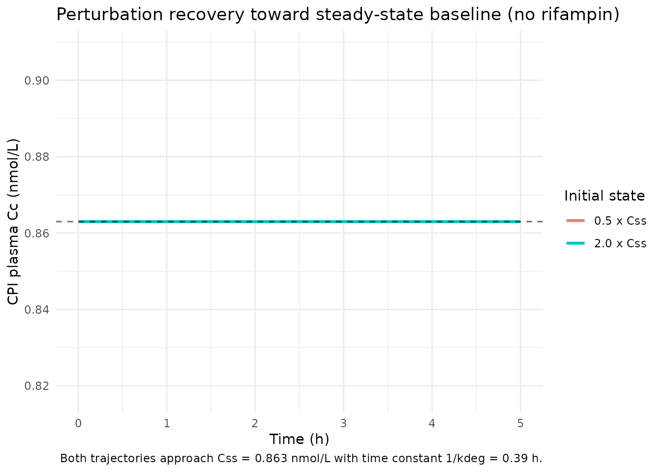
Inhibition response (model algebra, constant perpetrator concentration)
At a sustained constant perpetrator concentration
CP_RIF_UM = Cinh, the new steady-state plasma CPI is
Css(Cinh) = Baseline * kdeg / kdeg_eff(Cinh) = Baseline / (fnh + (1 - fnh) / (1 + Cinh / Ki,u)).
This is a property of the model algebra itself (no time-course is
involved); the figure below shows the inhibition response curve over a
range of constant Cinh values spanning unbound concentrations typical of
a 600 mg oral rifampin dose. This is not a reproduction
of the original Yoshida 2018 fit – the original used a time-varying
Simcyp-predicted portal-vein profile that is not reproducible from
on-disk sources.
fnh <- 0.129
kiu <- 0.0203
baseline <- 0.863

cinh_grid <- 10 ^ seq(-4, 2, length.out = 100)
css_grid  <- baseline / (fnh + (1 - fnh) / (1 + cinh_grid / kiu))
ratio_grid <- css_grid / baseline

inhib_df <- data.frame(cinh = cinh_grid, css = css_grid, ratio = ratio_grid)
ggplot(inhib_df, aes(cinh, ratio)) +
  geom_line(linewidth = 1) +
  scale_x_log10() +
  geom_hline(yintercept = 1 / fnh, linetype = "dashed", alpha = 0.6) +
  geom_vline(xintercept = kiu, linetype = "dotted", alpha = 0.6) +
  labs(x = "Sustained rifampin unbound portal-vein concentration (umol/L, log scale)",
       y = "Steady-state CPI ratio (Css / Baseline)",
       title = "Yoshida 2018 RIF-CPI inhibition response (algebra-only)",
       caption = paste0(
         "Dotted vertical line: Ki,u = ", kiu, " umol/L; ",
         "dashed horizontal asymptote: 1 / fNH = ", round(1 / fnh, 2),
         " (complete hepatic inhibition).")) +
  theme_minimal()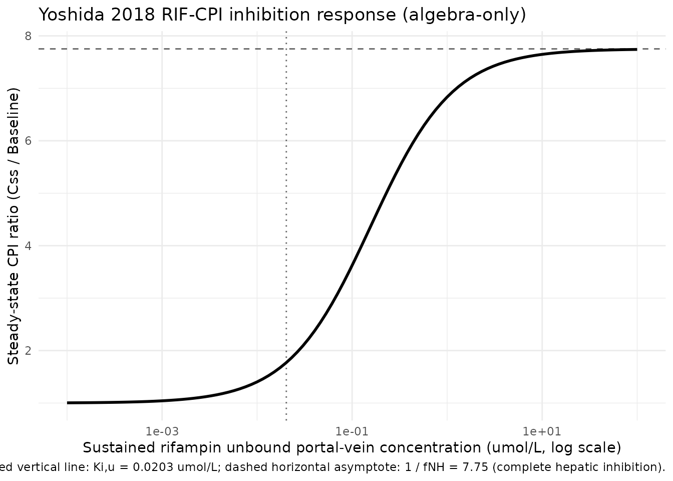
The asymptotic upper bound 1 / fNH = 7.75 is the maximum
CPI fold-increase under complete OATP1B inhibition; any finite Cinh
produces a smaller fold-increase. This is a structural consequence of
fNH > 0 (a non-zero non-hepatic clearance pathway remains active
regardless of OATP1B inhibition) and is why the paper’s sensitivity
analysis showed that smaller fNH estimates produce larger Ki,u
estimates.
Mass-balance check at the analytic baseline
At steady state with no inhibitor, the production rate
ksyn = kdeg * Baseline = 2.55 * 0.863 = 2.2007 nmol/L/h
must exactly balance the elimination rate
kdeg * Css = 2.55 * 0.863 = 2.2007 nmol/L/h:
kdeg <- 2.55
baseline <- 0.863
ksyn <- kdeg * baseline
elim_rate <- kdeg * baseline
cat("Production rate  :", round(ksyn, 6),      "nmol/L/h\n")
#> Production rate  : 2.20065 nmol/L/h
cat("Elimination rate :", round(elim_rate, 6), "nmol/L/h\n")
#> Elimination rate : 2.20065 nmol/L/h
stopifnot(abs(ksyn - elim_rate) < 1e-9)
Comparison against published values
| Quantity | Yoshida 2018 reported value | Simulated typical-value |
|---|---|---|
| Baseline plasma CPI (Css) | 0.863 nmol/L (Table 2) | 0.863 nmol/L |
| Asymptotic max CPI fold-increase (1/fNH) | 7.75 (derived from fNH = 12.9 %) | 7.75 |
| Ki,u rifampin | 0.0203 umol/L (Table 2) | (input parameter) |
Yoshida 2018 does not tabulate Cmax / AUC for the CPI plasma profile under rifampin – the validation in the paper is a visual predictive check against the observed plasma concentration vs time profile (Figure 2a). Without the Simcyp portal-vein rifampin concentration profile (see Assumptions and deviations) the original time-course cannot be reproduced.
Assumptions and deviations
-
Simcyp portal-vein rifampin concentration not
reproducible. Yoshida 2018 used the Simcyp v16r1 default
single-dose rifampin model file as the forcing function for
CP_RIF_UM; that PBPK output is not on disk and is not reproducible from open sources. Per the operator’s instruction for this extraction, the vignette intentionally does not approximate the rifampin PK with an analytic surrogate. Users wishing to reproduce the original CPI time-course must supply their own portal-vein unbound rifampin profile (e.g., from a registered nlmixr2lib rifampicin model such asmodellib('Barnett_2018_rifampicin'), after MW conversion to umol/L; note that the Barnett profile differs in shape from the Simcyp default profile, so the resulting CPI excursion will be quantitatively different). - Ki,u is conditional on the perpetrator-PK model. Yoshida 2018 Discussion documents that a preliminary refit using an updated rifampin model that matched observed Cmax / half-life produced an estimated Ki,u of 0.13 umol/L (about 5x higher than the 0.0203 umol/L reported in Table 2 and encoded here). Downstream users should treat the encoded Ki,u as a fit-conditional estimate rather than a fundamental property of rifampin.
-
No IIV. Table 2 reports no IIV for the rifampin-CPI
fit (
-in the IIV rows). The model encodes only typical-value parameters; users running stochastic simulations would need to supply external variability assumptions. - fNH is bounded but lightly identified. The paper’s sensitivity analysis (Figure 3a) shows that the overall model fit is not strongly sensitive to fNH, but Ki,u and kdeg do vary substantially with fNH (Ki,u can reach 10x the Table 2 value when fNH is forced to 0). The independent estimate of fNH from urinary CPI in Rotor’s-syndrome patients (paper Table 1, geometric mean approximately 9.8 %) is consistent with the model-estimated 12.9 % to within a factor of about 1.3, lending external support to the encoded value.
-
No explicit volume of distribution. Yoshida 2018’s
one-compartment parameterisation operates directly on the plasma
concentration (no
Vcappears), in contrast to the sibling Barnett 2018 CPI model (modellib('Barnett_2018_coproporphyrin_I')) which uses an explicitVcpi. This is a structural choice in the original paper, not a deviation. - Demographics not tabulated. Yoshida 2018 does not tabulate per-subject body-weight / age data for the rifampin-CPI cohort; the demographics block reflects only what is inferable from the cited Lai et al. 2016 source clinical study.