Coproporphyrin I (Yoshida 2018, GDC-0810)
Source:vignettes/articles/Yoshida_2018_coproporphyrin_I_GDC0810.Rmd
Yoshida_2018_coproporphyrin_I_GDC0810.RmdModel and source
- Citation: Yoshida K, Guo C, Sane R. Quantitative Prediction of OATP-Mediated Drug-Drug Interactions With Model-Based Analysis of Endogenous Biomarker Kinetics. CPT Pharmacometrics Syst. Pharmacol. 2018;7(8):517-524. doi:10.1002/psp4.12315. The GDC-0810-CPI calibration (Table 2 right column) was fit to the Liu et al. 2018 plasma CPI profile cohort using portal-vein GDC-0810 concentrations from an in-house Y. Chen et al. PBPK model (cited as personal communication; not on disk), so users must supply CP_GDC_UM externally. The companion rifampin calibration is parameterised in modellib(‘Yoshida_2018_coproporphyrin_I_rifampin’).
- Description: One-compartment endogenous turnover model for the OATP1B-substrate biomarker coproporphyrin I (CPI) in healthy adults (Yoshida 2018, GDC-0810-CPI calibration). CPI is produced at a zero-order synthesis rate Ksyn = kdeg * Baseline and eliminated as a single first-order pool whose overall rate constant kdeg is decomposed into a non-hepatic fraction fNH (held fixed at 12.9 %, unaffected by inhibitor) and a hepatic fraction 1 - fNH (competitively inhibited by the OATP1B perpetrator via Ki,u). The perpetrator portal-vein unbound concentration enters as a time-varying covariate CP_GDC_UM (umol/L); setting CP_GDC_UM = 0 collapses the model to the inhibitor-free steady state Baseline. This file encodes the GDC-0810-CPI calibration (Table 2 right column) with IIV on Baseline (18.2 %CV) and Ki,u (30.1 %CV); a sibling file Yoshida_2018_coproporphyrin_I_rifampin encodes the rifampin calibration with its own Ki,u, kdeg, and no IIV. The original fit used a Y. Chen et al. in-house PBPK model for GDC-0810 portal-vein concentrations (personal communication, not on disk and not in the nlmixr2lib registry), so downstream users must supply CP_GDC_UM externally.
- Article: https://doi.org/10.1002/psp4.12315
Population and biological context
Coproporphyrin I (CPI) is a heme-biosynthesis byproduct and a
selective endogenous substrate of the hepatic OATP1B1 / OATP1B3
transporters. Yoshida 2018 proposed a simple one-compartment turnover
model for plasma CPI in which the overall first-order degradation rate
constant kdeg is split into a non-hepatic fraction
fNH (unaffected by perpetrator) and a hepatic fraction
1 - fNH that is competitively inhibited by the OATP1B
perpetrator via the unbound inhibition constant Ki,u. The
synthesis rate is anchored to the steady-state identity
Ksyn = kdeg * Baseline.
This file encodes the GDC-0810-CPI calibration (Table 2 right
column). The underlying clinical dataset is the Liu et al. 2018 cohort
(healthy adult female subjects; GDC-0810 was administered orally as the
OATP1B perpetrator). The original fit used an in-house Y. Chen et
al. PBPK model for portal-vein unbound GDC-0810 concentrations as the
forcing function. In contrast to the rifampin-CPI calibration
(modellib('Yoshida_2018_coproporphyrin_I_rifampin')), this
fit (i) holds fNH FIXED at 12.9 % (the rifampin-CPI estimate) and (ii)
reports IIV on Baseline (18.2 %CV) and on Ki,u (30.1 %CV).
The same context is available programmatically via
readModelDb("Yoshida_2018_coproporphyrin_I_GDC0810")$population.
Source trace
| Equation / parameter | Value | Source location |
|---|---|---|
lrbase |
log(0.873) | Yoshida 2018 Table 2, GDC-0810-CPI column ‘Baseline (nM)’ = 0.873 (RSE 7.47%) |
lkdeg |
log(1.25) | Yoshida 2018 Table 2, GDC-0810-CPI column ‘kdeg (1/h)’ = 1.25 (RSE 5.88%) |
logitfnh |
fixed(qlogis(0.129)) | Yoshida 2018 Table 2, GDC-0810-CPI column ‘fNH’ = 12.9 % FIXED |
lkiu |
log(0.00174) | Yoshida 2018 Table 2, GDC-0810-CPI column ‘Ki,u (uM)’ = 0.00174 (RSE 27.3%) |
etalrbase |
0.03244 | Yoshida 2018 Table 2, GDC-0810-CPI column ‘IIV on Baseline’ = 18.2 %CV; log(1 + 0.182^2) |
etalkiu |
0.08660 | Yoshida 2018 Table 2, GDC-0810-CPI column ‘IIV on Ki,u’ = 30.1 %CV; log(1 + 0.301^2) |
propSd |
0.119 | Yoshida 2018 Table 2, GDC-0810-CPI column ‘Proportional residual error’ = 11.9 %CV |
| ODE form | n/a | Yoshida 2018 Methods (Model-based analysis with inhibitor kinetics) and Figure S1b |
| Steady-state baseline (analytic) | Ksyn / kdeg = Baseline |
Derived from d(Cc)/dt = 0 with no inhibitor:
Cc_ss = Baseline = 0.873 nmol/L
|
Units of every ODE term (dimensional analysis)
The Yoshida 2018 parameterisation operates directly on the plasma CPI
concentration (there is no explicit volume of distribution). The state
variable central carries the same units as Cc
(nmol/L); ksyn and the elimination flux therefore both have
units of nmol/L/h.
Term in d/dt(central) = ksyn - kdeg_eff * central
|
Units |
|---|---|
central (state) and Cc
|
nmol/L |
kdeg and kdeg_eff
|
1/h |
ksyn = kdeg * rbase |
nmol/L/h |
kdeg_eff * central |
nmol/L/h |
d/dt(central) |
nmol/L/h ok |
Steady-state check (no GDC-0810, deterministic typical-value)
With CP_GDC_UM = 0 the inhibition term collapses to
kdeg_eff = kdeg and the analytic steady-state plasma CPI is
Baseline = 0.873 nmol/L. The simulator should hold this
value indefinitely.
mod <- readModelDb("Yoshida_2018_coproporphyrin_I_GDC0810")
mod_typical <- rxode2::zeroRe(mod)

make_cpi_events <- function(t_end = 200, dt = 2, cgdc = 0) {
  data.frame(
    id   = 1L,
    time = seq(0, t_end, by = dt),
    evid = 0L,
    amt  = 0,
    cmt  = "Cc",
    CP_GDC_UM = cgdc
  )
}

ss_sim <- rxode2::rxSolve(mod_typical, events = make_cpi_events(t_end = 200))
#> ℹ omega/sigma items treated as zero: 'etalrbase', 'etalkiu'
cat("Yoshida 2018 (GDC-0810-CPI) typical-value baseline (no GDC-0810):\n")
#> Yoshida 2018 (GDC-0810-CPI) typical-value baseline (no GDC-0810):
cat("  Cc(t = 0)  :", round(ss_sim$Cc[1], 4), "nmol/L\n")
#>   Cc(t = 0)  : 0.873 nmol/L
cat("  Cc(t = 200):", round(tail(ss_sim$Cc, 1), 4), "nmol/L\n")
#>   Cc(t = 200): 0.873 nmol/L
cat("  Drift over 200 h:", signif(diff(range(ss_sim$Cc)), 3), "nmol/L\n")
#>   Drift over 200 h: 0 nmol/L
cat("  Analytic Css (= Baseline):", 0.873, "nmol/L\n")
#>   Analytic Css (= Baseline): 0.873 nmol/L
stopifnot(diff(range(ss_sim$Cc)) < 1e-6)
Perturbation-recovery (no GDC-0810, displaced initial condition)
Displacing the central state away from the steady-state value should
give a monotone first-order recovery toward Baseline with time constant
1 / kdeg = 1 / 1.25 = 0.80 h.
ev <- make_cpi_events(t_end = 8, dt = 0.1, cgdc = 0)

sim_low  <- rxode2::rxSolve(mod_typical, events = ev,
                            inits = c(central = 0.5 * 0.873))
#> ℹ omega/sigma items treated as zero: 'etalrbase', 'etalkiu'
sim_high <- rxode2::rxSolve(mod_typical, events = ev,
                            inits = c(central = 2.0 * 0.873))
#> ℹ omega/sigma items treated as zero: 'etalrbase', 'etalkiu'

cat("Perturbation recovery toward Css = 0.873 nmol/L:\n")
#> Perturbation recovery toward Css = 0.873 nmol/L:
cat("  Start 0.5x :", round(sim_low$Cc[1], 4),
    "  End:", round(tail(sim_low$Cc, 1), 4), "nmol/L\n")
#>   Start 0.5x : 0.873   End: 0.873 nmol/L
cat("  Start 2.0x :", round(sim_high$Cc[1], 4),
    "  End:", round(tail(sim_high$Cc, 1), 4), "nmol/L\n")
#>   Start 2.0x : 0.873   End: 0.873 nmol/L

t_4tau <- 4 / 1.25
sim_4tau_low <- rxode2::rxSolve(mod_typical,
  events = data.frame(id = 1L, time = c(0, t_4tau), evid = 0L,
                       amt = 0, cmt = "Cc", CP_GDC_UM = 0),
  inits = c(central = 0.5 * 0.873))
#> ℹ omega/sigma items treated as zero: 'etalrbase', 'etalkiu'
cat("  After 4 / kdeg = ", round(t_4tau, 3), " h from 0.5x start: Cc =",
    round(tail(sim_4tau_low$Cc, 1), 4), "nmol/L (within 2% of Css)\n")
#>   After 4 / kdeg =  3.2  h from 0.5x start: Cc = 0.873 nmol/L (within 2% of Css)
recovery <- dplyr::bind_rows(
  sim_low  |> as.data.frame() |> dplyr::mutate(start = "0.5 x Css"),
  sim_high |> as.data.frame() |> dplyr::mutate(start = "2.0 x Css")
)
ggplot(recovery, aes(time, Cc, colour = start)) +
  geom_line(linewidth = 1) +
  geom_hline(yintercept = 0.873, linetype = "dashed", alpha = 0.6) +
  labs(x = "Time (h)", y = "CPI plasma Cc (nmol/L)",
       title = "Perturbation recovery toward steady-state baseline (no GDC-0810)",
       colour = "Initial state",
       caption = "Both trajectories approach Css = 0.873 nmol/L with time constant 1/kdeg = 0.80 h.") +
  theme_minimal()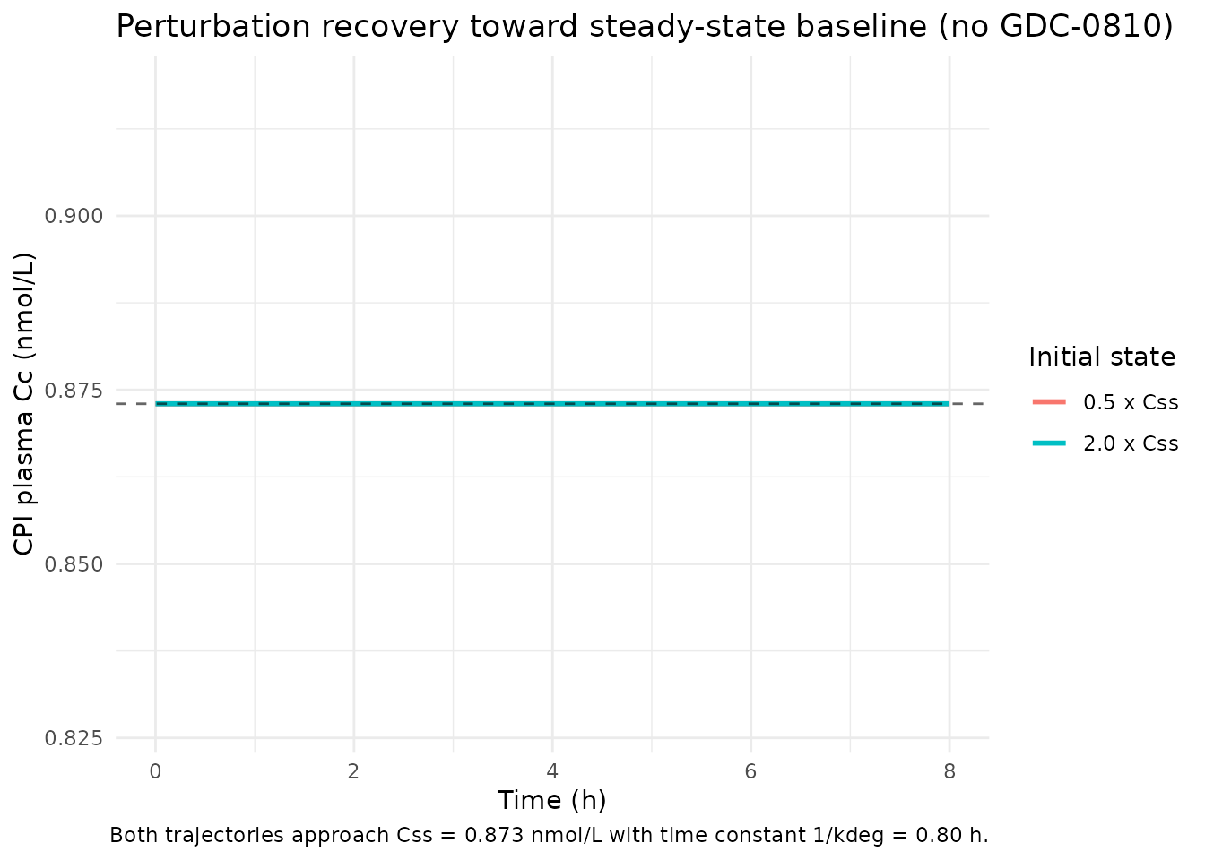
Inhibition response (model algebra, constant perpetrator concentration)
At a sustained constant perpetrator concentration
CP_GDC_UM = Cinh, the new steady-state plasma CPI is
Css(Cinh) = Baseline / (fnh + (1 - fnh) / (1 + Cinh / Ki,u)).
This is a property of the model algebra itself (no time-course is
involved). The encoded GDC-0810 Ki,u (0.00174 umol/L) is about 12x lower
than the rifampin Ki,u (0.0203 umol/L) on an unbound basis, consistent
with GDC-0810 being a more potent OATP1B inhibitor at equivalent unbound
concentrations. This is not a reproduction of the
original Yoshida 2018 fit – the original used a time-varying in-house
PBPK GDC-0810 portal-vein profile that is not reproducible from on-disk
sources.
fnh <- 0.129
kiu <- 0.00174
baseline <- 0.873

cinh_grid <- 10 ^ seq(-6, 1, length.out = 100)
css_grid  <- baseline / (fnh + (1 - fnh) / (1 + cinh_grid / kiu))
ratio_grid <- css_grid / baseline

inhib_df <- data.frame(cinh = cinh_grid, css = css_grid, ratio = ratio_grid)
ggplot(inhib_df, aes(cinh, ratio)) +
  geom_line(linewidth = 1) +
  scale_x_log10() +
  geom_hline(yintercept = 1 / fnh, linetype = "dashed", alpha = 0.6) +
  geom_vline(xintercept = kiu, linetype = "dotted", alpha = 0.6) +
  labs(x = "Sustained GDC-0810 unbound portal-vein concentration (umol/L, log scale)",
       y = "Steady-state CPI ratio (Css / Baseline)",
       title = "Yoshida 2018 GDC-0810-CPI inhibition response (algebra-only)",
       caption = paste0(
         "Dotted vertical line: Ki,u = ", kiu, " umol/L; ",
         "dashed horizontal asymptote: 1 / fNH = ", round(1 / fnh, 2),
         " (complete hepatic inhibition).")) +
  theme_minimal()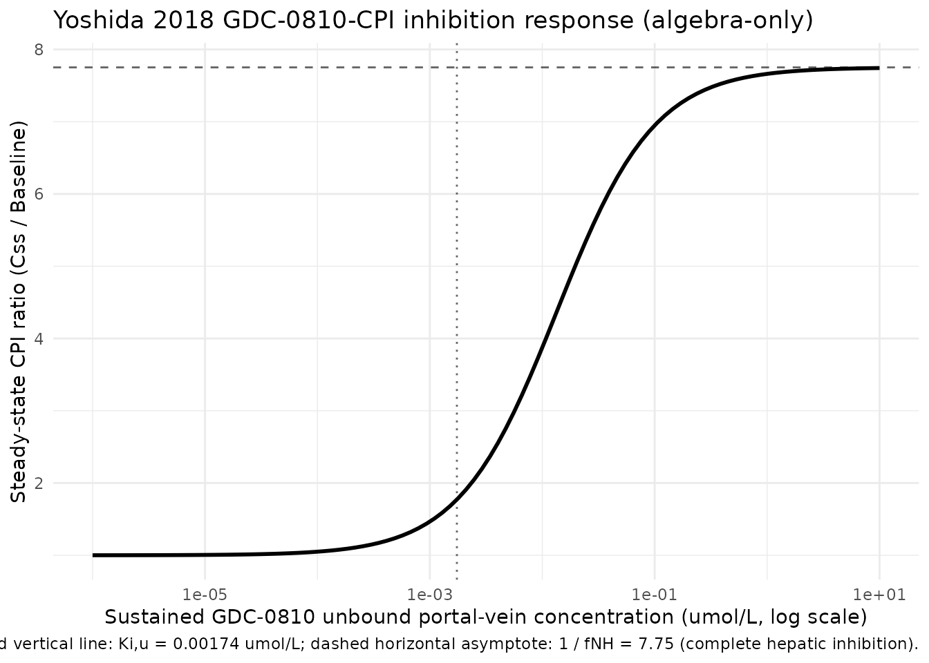
The asymptotic upper bound 1 / fNH = 7.75 (identical to
the rifampin-CPI sibling because fNH is fixed at the same value) is the
maximum CPI fold-increase under complete OATP1B inhibition; any finite
Cinh produces a smaller fold-increase.
Mass-balance check at the analytic baseline
At steady state with no inhibitor, the production rate
ksyn = kdeg * Baseline = 1.25 * 0.873 = 1.0913 nmol/L/h
must exactly balance the elimination rate:
kdeg <- 1.25
baseline <- 0.873
ksyn <- kdeg * baseline
elim_rate <- kdeg * baseline
cat("Production rate  :", round(ksyn, 6),      "nmol/L/h\n")
#> Production rate  : 1.09125 nmol/L/h
cat("Elimination rate :", round(elim_rate, 6), "nmol/L/h\n")
#> Elimination rate : 1.09125 nmol/L/h
stopifnot(abs(ksyn - elim_rate) < 1e-9)
Stochastic IIV demonstration (no GDC-0810, steady-state Cc)
The GDC-0810-CPI fit reports IIV on Baseline (18.2 %CV) and on Ki,u
(30.1 %CV). Simulating 200 virtual subjects at
CP_GDC_UM = 0 should reproduce the Baseline 18.2 %CV; Ki,u
IIV does not influence Cc when Cinh = 0 (the inhibition term is the
identity).
set.seed(20260530)
mod_iiv <- readModelDb("Yoshida_2018_coproporphyrin_I_GDC0810")

ev_iiv <- expand.grid(id = 1:200, time = c(0, 10)) |>
  dplyr::arrange(id, time) |>
  dplyr::mutate(evid = 0L, amt = 0, cmt = "Cc", CP_GDC_UM = 0)

sim_iiv <- rxode2::rxSolve(mod_iiv, events = ev_iiv) |> as.data.frame()
css_per_id <- sim_iiv |>
  dplyr::filter(time == 10) |>
  dplyr::pull(Cc)

cv_obs <- 100 * sd(css_per_id) / mean(css_per_id)
cat("Stochastic Baseline simulation (n = 200, CP_GDC_UM = 0):\n")
#> Stochastic Baseline simulation (n = 200, CP_GDC_UM = 0):
cat("  Mean Css :", round(mean(css_per_id), 4), "nmol/L (target", 0.873, ")\n")
#>   Mean Css : 0.8892 nmol/L (target 0.873 )
cat("  CV%      :", round(cv_obs, 1), "%  (target 18.2 %)\n")
#>   CV%      : 18.7 %  (target 18.2 %)
Comparison against published values
| Quantity | Yoshida 2018 reported value | Simulated typical-value |
|---|---|---|
| Baseline plasma CPI (Css) | 0.873 nmol/L (Table 2) | 0.873 nmol/L |
| Asymptotic max CPI fold-increase (1/fNH) | 7.75 (derived from fNH = 12.9 %) | 7.75 |
| Ki,u GDC-0810 | 0.00174 umol/L (Table 2) | (input parameter) |
| IIV on Baseline | 18.2 %CV (Table 2) | reproduced stochastically above |
Yoshida 2018 reports VPC plots of plasma CPI under GDC-0810 (Figure 2b) but does not tabulate Cmax / AUC; without the in-house GDC-0810 PBPK profile (see Assumptions and deviations) the original time-course cannot be reproduced.
Assumptions and deviations
-
In-house GDC-0810 PBPK profile not reproducible.
Yoshida 2018 used an unpublished Y. Chen et al. PBPK model for GDC-0810
(cited as personal communication in the paper Methods) as the forcing
function for
CP_GDC_UM; that PBPK output is not on disk and no GDC-0810 PK model is currently registered in nlmixr2lib. Per the operator’s instruction for this extraction, the vignette intentionally does not approximate the GDC-0810 PK with an analytic surrogate. Users wishing to reproduce the original CPI time-course must supply their own portal-vein unbound GDC-0810 profile. -
fNH is FIXED at the rifampin-CPI estimate. Table 2
fixes fNH at 12.9 % for the GDC-0810-CPI fit (the value estimated from
the rifampin-CPI analysis). The paper’s sensitivity analysis (Figure 3b)
shows fNH has small influence on the other GDC-0810 parameters,
justifying the fix. Downstream users re-fitting this model should
consider whether to free fNH; the model file uses
fixed()to mark the structural assumption. - Ki,u IIV partly reflects perpetrator-exposure variability. Yoshida 2018 Discussion notes that observed GDC-0810 plasma AUC IIV was about 20 %CV; the encoded 30.1 %CV IIV on Ki,u therefore includes per-subject variability in portal-vein GDC-0810 exposure in addition to intrinsic Ki,u variability. Users who do supply a GDC-0810 PK profile with subject-level IIV may double-count this variability source.
- Cohort is female-only. The Liu et al. 2018 underlying clinical dataset enrolled healthy adult female subjects (consistent with GDC-0810 being a selective estrogen receptor downregulator). Per-subject demographic details are not tabulated by Yoshida 2018.
-
No explicit volume of distribution. Yoshida 2018’s
one-compartment parameterisation operates directly on the plasma
concentration (no
Vcappears), in contrast to the sibling Barnett 2018 CPI model (modellib('Barnett_2018_coproporphyrin_I')). -
kdegdiffers from the rifampin-CPI fit. Table 2 reportskdeg= 1.25 1/h for GDC-0810-CPI vs 2.55 1/h for RIF-CPI; the paper describes these as “comparable” although the values differ approximately 2-fold. The difference may reflect dataset / fit-specific factors (e.g., differences in perpetrator-PK model identifiability between the two cohorts).