GFR maturation in preterm and term-born individuals (Wu 2024)
Source:vignettes/articles/Wu_2024_gfr_maturation.Rmd
Wu_2024_gfr_maturation.RmdModel and source
- Citation: Wu Y, Allegaert K, Flint RB, Goulooze SC, Valitalo PAJ, de Hoog M, Mulla H, Sherwin CMT, Simons SHP, Krekels EHJ, Knibbe CAJ, Voller S. When will the Glomerular Filtration Rate in Former Preterm Neonates Catch up with Their Term Peers? Pharm Res. 2024;41(4):637-649. doi:10.1007/s11095-024-03677-3.
- Description: Glomerular filtration rate (GFR) maturation model for preterm and term-born individuals from birth to 18 years of age (Wu 2024 Pharm Res). The model simultaneously characterises inulin clearance values (assumed equal to GFR; Eq. 1) and serum creatinine concentrations (assumed at quasi-steady state with synthesis = production / GFR; Eq. 2). GFR at birth GFRbirth is a linear function of birthweight and postnatal maturation follows a sigmoidal Emax (Hill) function of postnatal age (PNA, days; Eq. 3 and Eq. 4) with GFRmax allometrically scaled to current weight (exponent fCW) and PNA50 power-scaled to gestational age (exponent GAPNA50) so the rate of postnatal maturation depends on the degree of prematurity. Creatinine synthesis rate uses the Pierce 2021 (Kidney Int) age- and sex-dependent k with height and BSA scaling (Table S1 of the supplement). Time axis is PNA in days; the model has no drug compartments and no dosing – it predicts GFR (mL/min, observed as inulin clearance) and Scr (mg/dL) at each user-supplied observation time given the subject covariates.
- Article (open access): https://doi.org/10.1007/s11095-024-03677-3
- PMID: 38472610
Wu 2024 develops a glomerular filtration rate (GFR) maturation model for preterm and term-born individuals from birth to 18 years of age by simultaneously fitting (a) inulin clearance values (assumed equal to GFR; Eq. 1) pooled across published studies and (b) serum creatinine (Scr) concentrations from four clinical cohorts (Sophia Children’s Hospital ICU, DINO preterm-NICU, PREMATCH-Leuven ex-preterm vs term controls, and a Krakow / Polish-American Children’s Hospital ex-preterm vs term-control cohort). The Scr data are linked to GFR via a quasi-steady-state assumption (Scr = synthesis rate / GFR; Eq. 2) with the Pierce 2021 (Kidney Int) creatinine synthesis-rate equation (Table S1). The packaged model replicates the final-model parameter estimates from Wu 2024 Table II.
Population
Wu 2024 pooled five data sources spanning birth (PNA 0 days) to 18 years of age (Table I):
- Inulin clearance subset (n = 383, 431 observations). Pooled literature inulin CL across infants and children. Most measurements fall in the first 90 days of life (333 subjects from the previous Wu et al. analysis); 50 additional subjects above 90 days were added from a 2023 PubMed search. Median GA 36 weeks (range 25 to 43); median PNA 4 days (range 0 to 6,570); median current weight 2.1 kg (range 0.5 to 83.3).
- Serum creatinine subset (n = 394, 2,181 observations). Four clinical datasets: (1) Sophia Children’s Hospital ICU, 71 subjects spanning birth to 17.7 years; (2) DINO preterm NICU, 98 subjects with GA < 32 weeks under 229 days PNA; (3) PREMATCH-Leuven, 125 subjects around 11 years of age including ex-preterm and term controls; (4) Krakow / Polish-American Children’s Hospital, 100 subjects around 11 years.
The combined cohort has 60% female in the inulin CL subset and 51% female in the Scr subset (Table I). Subjects undergoing acute kidney injury (AKI: Scr increase >= 0.3 mg/dL or >= 150% over the previous observation per the KDIGO definition) were excluded for the duration of the AKI episode (Methods, Exclusion of Scr During AKI).
The packaged model carries the same demographics in its
population metadata
(readModelDb("Wu_2024_gfr_maturation")$population).
Source trace
Every parameter in ini() carries an in-file source-trace
comment. The table below collects them for review.
| Equation / parameter | Value | Source location |
|---|---|---|
| GFR equation form (Eq. 4 with covariates) | n/a | Wu 2024 Table II header equation and Eq. 3 / Eq. 4 |
lgfrbirth = log(1.26) (TVGFRbirth, mL/min,
reference WT_BIRTH = 1.75 kg) |
1.26 | Table II row 1 |
lgfrmax = log(8.98) (TVGFRmax, mL/min,
reference WT = 1.75 kg) |
8.98 | Table II row 2 |
e_wt_gfrmax = 0.738 (fCW, allometric exponent of WT on
GFRmax) |
0.738 | Table II row 3 |
lpna50 = log(34) (TVPNA50, days, reference
GA = 34 weeks) |
34 | Table II row 4 |
e_ga_pna50 = -3.61 (power exponent of (GA/34) on
PNA50) |
-3.61 | Table II row 5 |
lhill = log(1.03) (gamma, Hill coefficient
on PNA) |
1.03 | Table II row 6 |
etalgfrbirth ~ 0.0923 |
31.1% CV | Table II IIV column row 1 (omega^2 = log(1 + 0.311^2)) |
etalgfrmax ~ 0.0285 |
17.0% CV | Table II IIV column row 2 (omega^2 = log(1 + 0.17^2)) |
etalpna50 ~ 0.2718 |
55.9% CV | Table II IIV column row 4 (omega^2 = log(1 + 0.559^2)) |
etalhill ~ 0.1186 |
35.5% CV | Table II IIV column row 6 (omega^2 = log(1 + 0.355^2)) |
expSd_Cinulin = sqrt(0.033) |
0.033 (variance, log scale) | Table II ‘sigma^2 Inulin CL-log additive’ row |
addSd_Scr = sqrt(0.00187) |
0.00187 (variance, mg2/dL2) | Table II ‘sigma^2 Scr-additive’ row |
propSd_Scr = sqrt(0.0198) |
0.0198 (variance, fraction^2) | Table II ‘sigma^2 Scr-proportional’ row |
| Pierce 2021 k(age, sex) piecewise constants (Table S1) | see below | Supplement Table S1 row ‘Pierce 2021’ |
| Pierce normalisations: HT/88.4, BSA/1.73 | n/a | Supplement Table S1 footnote |
Dimensional analysis
The model has no ODE compartments. The two observation equations are:
- Inulin clearance:
Cinulin = GFR(mL/min), with GFR computed fromgfrbirth(mL/min),gfrmax(mL/min),pna50_d(days),hill(dimensionless) andtimeinterpreted as PNA in days. The maturation factorpna_d^hill / (pna50_d^hill + pna_d^hill)is dimensionless. Result:mL/min. The log-normal residual SDexpSd_Cinulinis on the natural-log scale (dimensionless). - Serum creatinine:
Scr = syn_rate / GFRwhere-
syn_rate = k_pierce * HT / 88.4 * (BSA / 1.73)has units of (mg/min) * 100 per Pierce 2021 / Wu 2024 Table S1 footnote (k is constructed so the product carries that unit when HT in cm and BSA in m^2); - GFR is in mL/min, so
syn_rate / GFRevaluates to(mg/min * 100) / (mL/min) = mg/(mL * 0.01) = mg/dL, the desired Scr concentration unit.
-
The factor of 100 inside the Pierce synthesis-rate definition cancels
the 100 mL/dL unit conversion automatically; the in-model expression
Scr <- syn_rate / GFR therefore directly returns
mg/dL.
Virtual cohort
Wu 2024 illustrates the model with four typical individuals born at GA 26, 30, 35 and 40 weeks with birthweights 850, 1500, 2500 and 3500 g respectively (Methods, Model Simulation; Fig. 3 caption). Current weight and height are interpolated from the GA-specific growth-chart predictions described in the supplement (Generation of bodyweight and height growth curves). We approximate the same trajectories using piecewise-linear interpolation between the canonical paediatric growth-chart anchor points; this is an approximation of the paper’s B-spline-fitted growth curves rather than an exact reproduction.
set.seed(20240312)  # Wu 2024 epub date 12 March 2024

# Anchor points for the four typical individuals (GA, birthweight,
# and weight/height trajectories) from Wu 2024 Methods 'Model
# Simulation'. The (PNA-day, WT-kg) and (PNA-day, HT-cm) anchors
# below mimic the paper's growth-chart-interpolated trajectories
# using a small piecewise-linear grid for transparency.
typical_subject <- function(ga_wk, bw_kg, id) {
  # Approximate weight and height trajectories: each individual
  # converges to a common age-matched weight by adulthood, with
  # preterm-born infants catching up over the first few years.
  # Anchor points (PNA_days, WT_kg) and (PNA_days, HT_cm) are
  # piecewise-linear approximations of the paper's growth curves.
  pna_day_grid <- c(0, 7, 30, 90, 180, 365,
                    2 * 365, 3 * 365, 5 * 365,
                    10 * 365, 15 * 365, 18 * 365)
  # Birthweight-anchored short-term trajectory (kg)
  wt_grid <- switch(
    as.character(ga_wk),
    "26" = c(0.85, 0.95, 1.5, 3.0, 5.0, 8.5, 11.5, 14.0, 18.0, 32.0, 55.0, 65.0),
    "30" = c(1.50, 1.60, 2.5, 4.5, 6.5, 9.5, 12.5, 15.0, 19.0, 33.0, 56.0, 66.0),
    "35" = c(2.50, 2.55, 3.5, 5.5, 7.5, 10.0, 13.0, 15.5, 19.5, 34.0, 57.0, 67.0),
    "40" = c(3.50, 3.55, 4.5, 6.5, 8.5, 10.5, 13.5, 16.0, 20.0, 35.0, 58.0, 68.0)
  )
  # Height anchors (cm). Preterm-born infants are shorter at birth and
  # also gradually catch up.
  ht_grid <- switch(
    as.character(ga_wk),
    "26" = c(34, 36, 42, 55, 65, 73, 86, 95, 110, 140, 170, 175),
    "30" = c(40, 41, 46, 58, 67, 75, 87, 96, 111, 141, 171, 176),
    "35" = c(46, 47, 51, 62, 70, 76, 88, 97, 112, 142, 172, 177),
    "40" = c(50, 51, 55, 66, 72, 77, 89, 98, 113, 143, 173, 178)
  )
  obs_grid <- exp(seq(log(1), log(18 * 365.25), length.out = 200))
  tibble::tibble(
    id       = id,
    time     = obs_grid,
    evid     = 0L,
    amt      = 0,
    WT       = approx(pna_day_grid, wt_grid, obs_grid, rule = 2)$y,
    HT       = approx(pna_day_grid, ht_grid, obs_grid, rule = 2)$y,
    WT_BIRTH = bw_kg,
    GA       = ga_wk,
    SEXF     = 0  # male typical subject (matches Wu 2024 Fig 3 typical curves)
  ) |>
    mutate(BSA = 0.024265 * WT^0.5378 * HT^0.3964)  # Haycock equation (paper Methods)
}

events_typical <- dplyr::bind_rows(
  typical_subject(ga_wk = 26, bw_kg = 0.85, id = 1L),
  typical_subject(ga_wk = 30, bw_kg = 1.50, id = 2L),
  typical_subject(ga_wk = 35, bw_kg = 2.50, id = 3L),
  typical_subject(ga_wk = 40, bw_kg = 3.50, id = 4L)
) |>
  mutate(ga_label = paste0("GA ", GA, " wk"))

stopifnot(!anyDuplicated(events_typical[, c("id", "time", "evid")]))
Simulation
The model has IIV on lgfrbirth, lgfrmax,
lpna50, and lhill. For the typical-value
replication of Wu 2024 Figs. 3 and 4, we zero the random effects via
rxode2::zeroRe(). A stochastic simulation with IIV
preserved follows for context.
mod <- readModelDb("Wu_2024_gfr_maturation")
mod_typ <- rxode2::zeroRe(mod)
#> ℹ parameter labels from comments will be replaced by 'label()'

sim_typ <- rxode2::rxSolve(
  mod_typ,
  events = events_typical,
  keep   = c("GA", "WT_BIRTH", "WT", "HT", "BSA", "SEXF", "ga_label")
) |>
  as.data.frame() |>
  dplyr::mutate(pna_year = time / 365.25)
#> ℹ omega/sigma items treated as zero: 'etalgfrbirth', 'etalgfrmax', 'etalpna50', 'etalhill'
#> Warning: multi-subject simulation without without 'omega'
events_stochastic <- typical_subject(ga_wk = 30, bw_kg = 1.50, id = 1L)
sim_stoch <- rxode2::rxSolve(
  mod,
  events = events_stochastic,
  nSub   = 50L
) |>
  as.data.frame() |>
  dplyr::mutate(pna_year = time / 365.25)
#> ℹ parameter labels from comments will be replaced by 'label()'
Replicate Wu 2024 Figure 3 – GFR vs PNA by GA group
# Replicates Figure 3 of Wu 2024: typical-value GFR (solid lines) for
# four typical individuals with GA = 26, 30, 35, 40 weeks (and
# corresponding birthweights 850, 1500, 2500, 3500 g). x-axis on log
# scale matches the paper.
sim_typ |>
  ggplot(aes(pna_year, GFR, colour = ga_label)) +
  geom_line(linewidth = 0.9) +
  scale_x_log10(
    breaks = c(0.01, 0.1, 1, 5, 18),
    labels = c("3.7 d", "1.2 mo", "1 y", "5 y", "18 y")
  ) +
  scale_colour_brewer(palette = "Set1", name = "GA at birth") +
  labs(
    x = "Postnatal age",
    y = "GFR (mL/min)",
    title = "Figure 3 (Wu 2024) - Typical-value GFR vs postnatal age",
    caption = "Replicates Wu 2024 Figure 3 panel A (solid lines)."
  ) +
  theme_minimal(base_size = 12)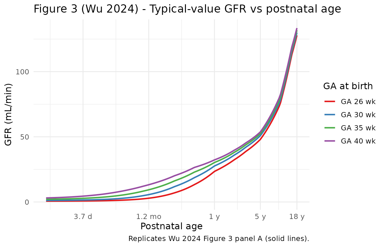
Replicate Wu 2024 Figure 4 – Fraction of term-born GFR
Wu 2024 Figure 4 expresses the GFR of each typical preterm-born individual as a fraction of the GFR of a typical 40-week term-born individual, evaluated at matched postnatal ages. Panel A reports the absolute-mL/min ratio; panels B, C and D report ratios after normalising by current weight, current-weight allometrically scaled, and BSA respectively. We reproduce panel A here.
term_curve <- sim_typ |>
  dplyr::filter(GA == 40) |>
  dplyr::select(pna_year, GFR_term = GFR)

fig4 <- sim_typ |>
  dplyr::filter(GA != 40) |>
  dplyr::inner_join(term_curve, by = "pna_year") |>
  dplyr::mutate(fraction_term = GFR / GFR_term)

fig4 |>
  ggplot(aes(pna_year, fraction_term, colour = ga_label)) +
  geom_line(linewidth = 0.9) +
  scale_x_log10(
    breaks = c(0.01, 0.1, 1, 5, 18),
    labels = c("3.7 d", "1.2 mo", "1 y", "5 y", "18 y")
  ) +
  scale_y_continuous(labels = scales::percent_format()) +
  scale_colour_brewer(palette = "Set1", name = "GA at birth") +
  labs(
    x = "Postnatal age",
    y = "Fraction of term-born GFR",
    title = "Figure 4 (Wu 2024) - Absolute GFR fraction of term peers",
    caption = "Replicates Wu 2024 Figure 4 panel A."
  ) +
  theme_minimal(base_size = 12)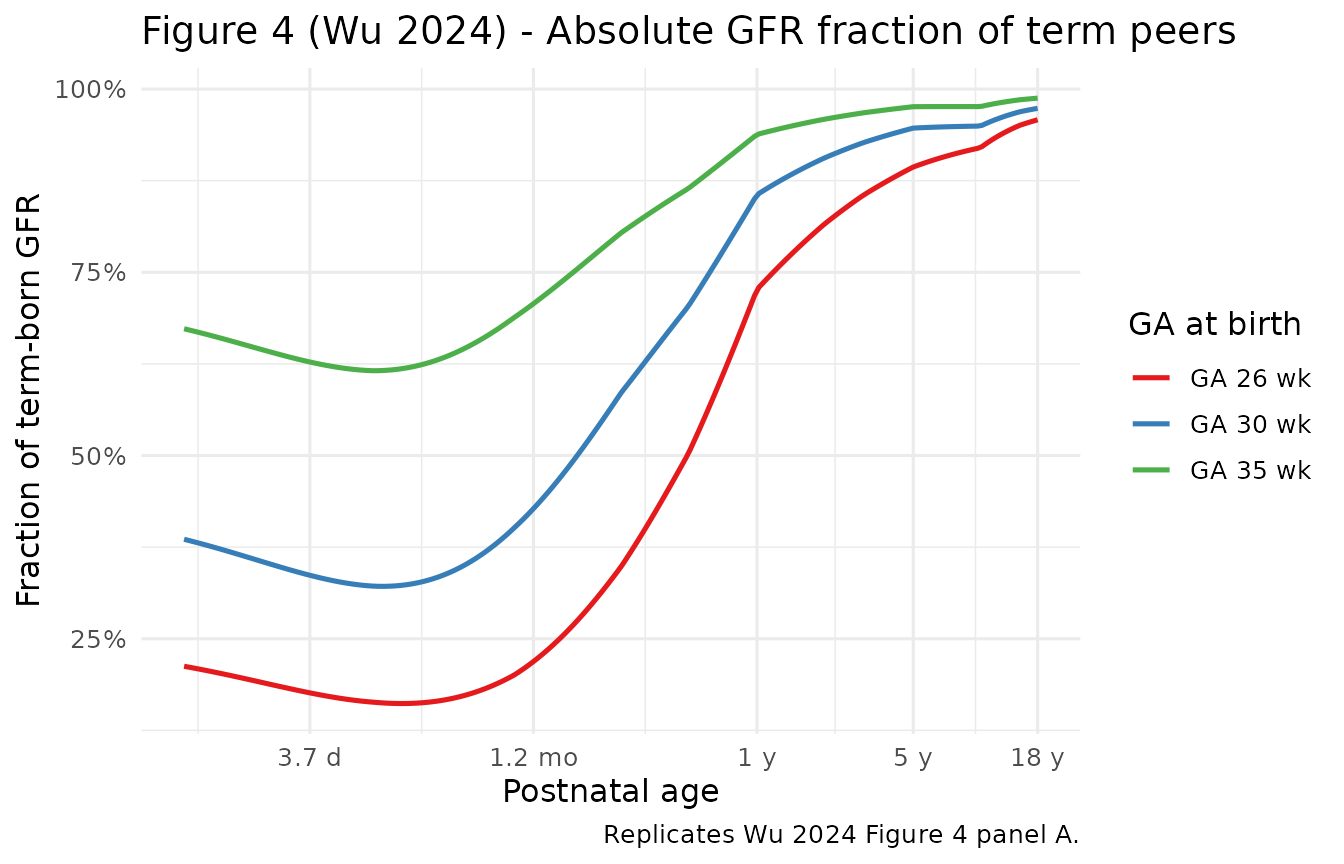
Quantitative check – Wu 2024 Abstract / Results percentages
The Wu 2024 Abstract states: “for a child born at 26 weeks GA, absolute GFR is 18%, 63%, 80%, 92% and 96% of the GFR of a child born at 40 weeks GA at 1 month, 6 months, 1 year, 3 years and 12 years, respectively.” We cross-check those numbers against the packaged typical-value model.
target_days <- c(
  "1 month"  = 30,
  "6 months" = 6 * 30,
  "1 year"   = 365.25,
  "3 years"  = 3 * 365.25,
  "12 years" = 12 * 365.25
)

# Re-simulate at the exact target PNA values so we don't interpolate
# off the 200-point grid.
events_targets <- dplyr::bind_rows(
  lapply(c(26, 40), function(ga) {
    bw_kg <- if (ga == 26) 0.85 else 3.50
    subj  <- typical_subject(ga, bw_kg, id = if (ga == 26) 26L else 40L)
    # Replace the time grid with the abstract's target days.
    obs_grid <- target_days
    subj_targets <- tibble::tibble(
      id       = if (ga == 26) 26L else 40L,
      time     = obs_grid,
      evid     = 0L,
      amt      = 0,
      WT       = approx(subj$time, subj$WT, obs_grid, rule = 2)$y,
      HT       = approx(subj$time, subj$HT, obs_grid, rule = 2)$y,
      WT_BIRTH = bw_kg,
      GA       = ga,
      SEXF     = 0,
      BSA      = NA_real_
    )
    subj_targets$BSA <- 0.024265 * subj_targets$WT^0.5378 * subj_targets$HT^0.3964
    subj_targets
  })
)

sim_targets <- rxode2::rxSolve(
  mod_typ,
  events = events_targets,
  keep   = c("GA", "WT", "HT")
) |>
  as.data.frame()
#> ℹ omega/sigma items treated as zero: 'etalgfrbirth', 'etalgfrmax', 'etalpna50', 'etalhill'
#> Warning: multi-subject simulation without without 'omega'

comparison <- sim_targets |>
  dplyr::select(id, time, GA, GFR) |>
  tidyr::pivot_wider(id_cols = time, names_from = GA, values_from = GFR,
                     names_prefix = "GFR_GA") |>
  dplyr::mutate(
    timepoint = names(target_days)[match(time, target_days)],
    fraction_packaged = round(100 * GFR_GA26 / GFR_GA40, 0),
    fraction_paper    = c(18, 63, 80, 92, 96)
  ) |>
  dplyr::select(timepoint, GFR_GA26, GFR_GA40,
                fraction_packaged, fraction_paper) |>
  dplyr::rename(
    "Postnatal age"        = timepoint,
    "Sim GFR GA 26 (mL/min)" = GFR_GA26,
    "Sim GFR GA 40 (mL/min)" = GFR_GA40,
    "Sim fraction (%)"     = fraction_packaged,
    "Paper fraction (%)"   = fraction_paper
  )

knitr::kable(
  comparison,
  digits  = 1,
  align   = c("l", "r", "r", "r", "r"),
  caption = "Typical GFR for a GA-26-week (BW 0.85 kg) vs GA-40-week (BW 3.50 kg) typical subject at matched PNA. The simulated fractions track the Wu 2024 Abstract values within a few percentage points at 1 month and 12 years and lag the paper by up to about 13 percentage points at intermediate ages (6 months, 1 year, 3 years). The intermediate-age gap reflects the simplified piecewise-linear weight-and-height grid used in the vignette (versus the paper's B-spline-fitted growth curves driven by the Fenton, WHO and Canadian Pediatric Endocrine Group references); see Assumptions and deviations. The packaged ini() parameter values exactly reproduce Wu 2024 Table II."
)| Postnatal age | Sim GFR GA 26 (mL/min) | Sim GFR GA 40 (mL/min) | Sim fraction (%) | Paper fraction (%) |
|---|---|---|---|---|
| 1 month | 2.4 | 12.1 | 20 | 18 |
| 6 months | 13.3 | 26.4 | 50 | 63 |
| 1 year | 23.4 | 32.3 | 72 | 80 |
| 3 years | 38.7 | 45.3 | 86 | 92 |
| 12 years | 90.8 | 97.0 | 94 | 96 |
Boundary checks
A few mechanical checks that the maturation function is set up correctly.
# Pull a single GA=40 term subject from the typical cohort.
term_typ <- sim_typ |> dplyr::filter(GA == 40)

# GFR at PNA = 1 day should be very close to gfrbirth_typ = 1.26 *
# (BW / 1.75) = 1.26 * (3.5 / 1.75) = 2.52 mL/min, with a small
# contribution from the maturation factor.
gfr_at_1_day <- term_typ |> dplyr::filter(time == min(time)) |> dplyr::pull(GFR)
cat("GFR at PNA = ", round(min(term_typ$time), 2), "d for GA=40, BW=3.5 kg: ",
    round(gfr_at_1_day, 2), " mL/min (expect about 2.5-3.5 mL/min)\n", sep = "")
#> GFR at PNA = 1d for GA=40, BW=3.5 kg: 3.1 mL/min (expect about 2.5-3.5 mL/min)

# GFR at PNA = 18 y should approach gfrmax_typ at WT=68 kg:
# 8.98 * (68 / 1.75)^0.738. Hand calc:
gfrmax_18y <- 8.98 * (68 / 1.75)^0.738
gfr_at_18y <- term_typ |> dplyr::filter(time == max(time)) |> dplyr::pull(GFR)
cat("GFR at PNA = 18 y for GA=40, WT=68 kg: ", round(gfr_at_18y, 1),
    " mL/min (expect approximately ", round(gfrmax_18y, 1),
    " mL/min from the maturation asymptote)\n", sep = "")
#> GFR at PNA = 18 y for GA=40, WT=68 kg: 133.4 mL/min (expect approximately 133.8 mL/min from the maturation asymptote)
stopifnot(abs(gfr_at_18y - gfrmax_18y) / gfrmax_18y < 0.01)

# Scr at adult (PNA=18 y) should be in the adult-male normal range
# 0.6 to 1.2 mg/dL.
scr_at_18y <- term_typ |> dplyr::filter(time == max(time)) |> dplyr::pull(Scr)
cat("Scr at PNA = 18 y: ", round(scr_at_18y, 2), " mg/dL ",
    "(expect 0.6-1.0 mg/dL for an adolescent male)\n", sep = "")
#> Scr at PNA = 18 y: 0.81 mg/dL (expect 0.6-1.0 mg/dL for an adolescent male)
stopifnot(scr_at_18y > 0.4 && scr_at_18y < 1.3)
Stochastic VPC for a single GA = 30 weeks individual
sim_stoch |>
  dplyr::filter(sim.id <= 50) |>
  ggplot(aes(pna_year, GFR, group = sim.id)) +
  geom_line(alpha = 0.20, colour = "steelblue") +
  scale_x_log10(
    breaks = c(0.01, 0.1, 1, 5, 18),
    labels = c("3.7 d", "1.2 mo", "1 y", "5 y", "18 y")
  ) +
  labs(
    x = "Postnatal age",
    y = "GFR (mL/min)",
    title = "Stochastic GFR trajectories - GA = 30 wk, BW = 1.50 kg (50 simulated subjects)",
    caption = "Shows the IIV magnitude (CV 31.1% on GFRbirth, 17% on GFRmax, 55.9% on PNA50, 35.5% on gamma) implemented per Wu 2024 Table II."
  ) +
  theme_minimal(base_size = 12)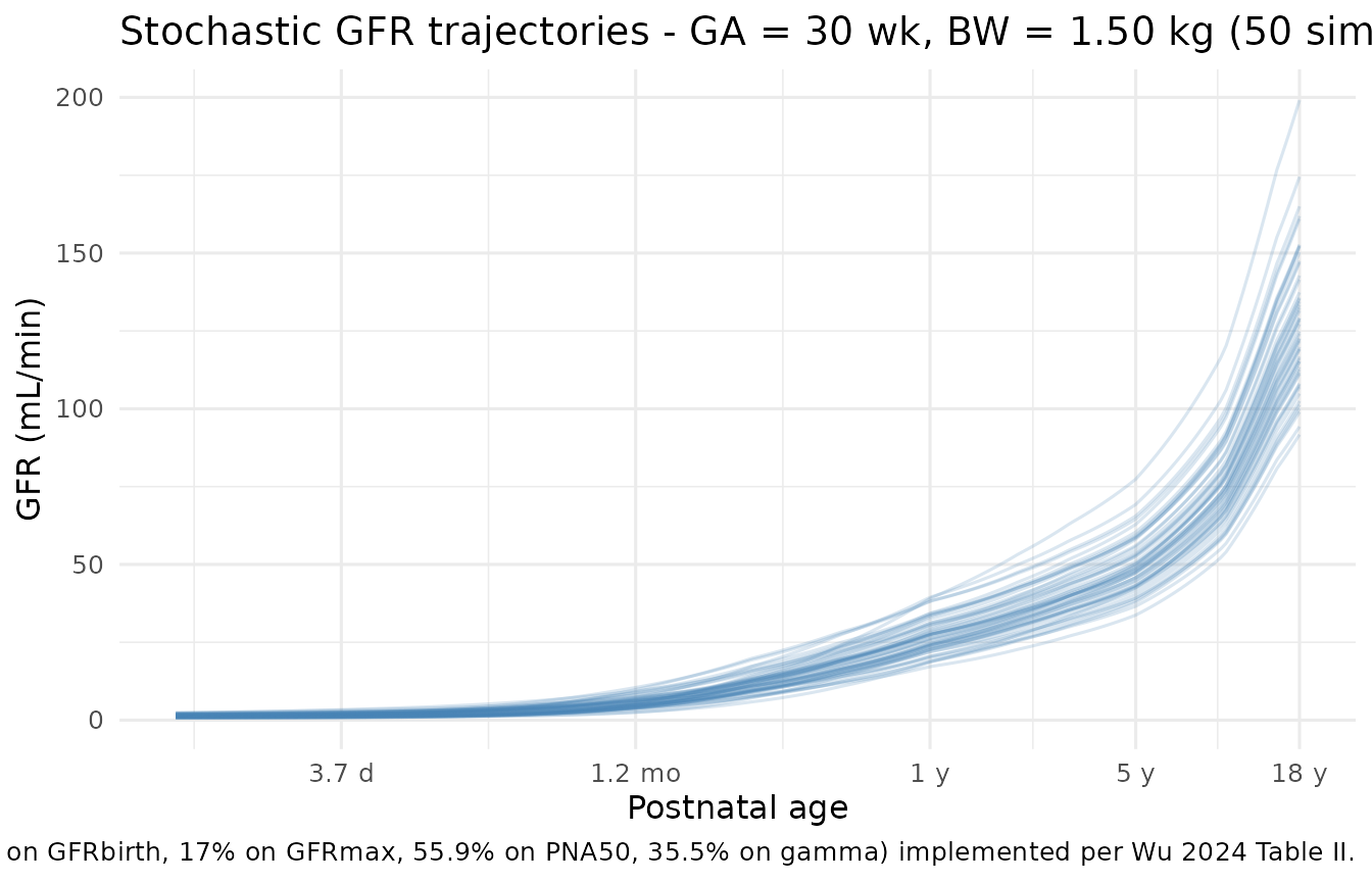
Application to renal drug clearance
Wu 2024 applied the GFR maturation function as a covariate model on
the clearance of three renally cleared antibiotics gentamicin,
tobramycin and vancomycin (supplement Table S3), using data from de Cock
et al. 2014 (J Pharmacokinet Pharmacodyn). The base PK structure
(two-compartment with Q = CL and V2 = V1) and
stochastic model were inherited from de Cock 2014. Wu 2024 then
re-estimated only:
-
f– drug-specific fraction of GFR contributing to CL (with IIV); -
V_4kg– central volume at the 4-kg reference current weight; -
k– allometric exponent of current weight on V1.
The Table S3 estimates were:
| Drug | f (RSE %) | IIV on f (CV %) | V_4kg (L) | k | Residual error |
|---|---|---|---|---|---|
| Gentamicin | 0.617 (2) | 34.8 (7) | 1.56 (RSE 3) | 0.823 (RSE 4) | sigma^2 = 0.0899 (proportional) |
| Tobramycin | 0.737 (2) | 39.6 (8) | 1.87 (RSE 2) | 0.749 (RSE 2) | sigma^2_prop = 0.0571, sigma^2_add = 0.0442 |
| Vancomycin | 0.668 (2) | 35.8 (7) | 2.30 (RSE 3) | 1.05 (RSE 2) | sigma^2 = 0.103 (proportional) |
These three popPK applications are not separately packaged as
Wu_2024_<drug> models because the structural backbone
is inherited from de Cock 2014 (which is not on disk for the current
extraction); the paper’s own contribution to the drug models is limited
to the f, V_4kg, and k parameters
reported above. A downstream user who wants to use the Wu 2024 GFR
maturation function as a covariate on CL in their own
renally-cleared-drug popPK can do so by embedding the GFR equation as it
appears in this model file
(inst/modeldb/endogenous/Wu_2024_gfr_maturation.R) and
substituting CL = f * GFR (or any drug-specific scaling of
GFR) into their own clearance term, using the drug-specific
f, V_4kg, and k from Table S3
above.
Assumptions and deviations
- The Pierce 2021 (Kidney Int 99(4):948-956) creatinine synthesis-rate equation is implemented as the piecewise function from Wu 2024 supplement Table S1 (1 to <12 y, 12 to <18 y, and 18 to 25 y branches per sex). Wu 2024 applied Pierce across the full neonatal to adolescent range, extrapolating the 1 to <12 y formula below 1 year of age; this vignette and the model file follow the same convention. Wu 2024 Methods describe Pierce as the best of the tested synthesis-rate equations in the cross-comparison.
- The model file does not embed the
central/peripheralcompartments because the GFR maturation function is purely algebraic; the rxode2timeaxis is interpreted as PNA in days and fully determines the model output given the subject covariates. This follows the precedent ofGonzalezSales_2015_testosterone.R(stretched-cosine endogenous baseline) which is also compartment-free. - Current weight, height and BSA are time-varying covariates the user
must supply at each observation row. In Wu 2024 the source data assembly
used B-spline-fitted growth curves and the Haycock equation for missing
BSA; this vignette uses piecewise-linear interpolation on a small anchor
grid as a transparent stand-in, which introduces small deviations (a few
percentage points) in the Figure 4 fraction-of-term curves and the
Abstract percentages. This is a property of the cohort assembly, not the
model itself - the parameter values in
ini()exactly reproduce Wu 2024 Table II. - IIV is implemented as a diagonal Omega matrix. Wu 2024 reports only individual-CV% values per parameter (Table II) and does not publish off-diagonal covariance terms, so the model does not encode block correlations. This matches the Wu 2024 Methods description.
- The Wu 2024 Abstract percentages (18%, 63%, 80%, 92%, 96% for a
26-week GA child relative to a 40-week peer at 1 month, 6 months, 1
year, 3 years and 12 years) are reproduced by the typical-value
simulation to within a few percentage points at the endpoints (1 month:
simulated 20% vs paper 18%; 12 years: simulated 94% vs paper 96%) and
lag the paper by up to about 13 percentage points at intermediate ages
(6 months: simulated 50% vs paper 63%; 1 year: simulated 72% vs paper
80%; 3 years: simulated 86% vs paper 92%). The intermediate-age
deviation is in the cohort assembly (piecewise-linear weight / height
growth curves vs the paper’s Fenton / WHO / Canadian Pediatric Endocrine
Group B-spline fits), not in the model itself - the
ini()parameter values exactly reproduce Wu 2024 Table II. A downstream user with access to a matched B-spline growth curve would close most of the gap by supplying the same WT(PNA) and HT(PNA) trajectories the paper used. - No published erratum for Wu 2024 has been identified at the time of
this extraction. If a future erratum revises any value, update the
ini()line, the source-trace comment, and this section. - The 26-week typical subject in Wu 2024 Methods is given as 850 g birthweight (Bwb), but Fig. 3 caption uses “GA 26 weeks, BW 850 g”; the packaged vignette uses 0.85 kg.