Caspofungin (Leshinsky 2017) -- cat
Source:vignettes/articles/Leshinsky_2017_caspofungin_cat.Rmd
Leshinsky_2017_caspofungin_cat.RmdModel and source
- Citation: Leshinsky J, McLachlan A, Foster DJR, Norris R, Barrs VR. Pharmacokinetics of caspofungin acetate to guide optimal dosing in cats. PLoS ONE. 2017;12(6):e0178783. doi:10.1371/journal.pone.0178783
- Description: Preclinical (cat). Two-compartment population PK model with first-order linear elimination from the central compartment for intravenous caspofungin acetate in healthy adult cats (Leshinsky 2017)
- Article (open access): doi:10.1371/journal.pone.0178783
Population
The model was developed from 8 healthy adult desexed domestic shorthair cats (4 females, 4 males) recruited from a research colony at Eurofins SCEC (Australia). Mean age was 3.94 +/- 1.84 years and mean body weight was 4.4 +/- 0.56 kg (Leshinsky 2017 Materials and methods, “Animals”). All cats had baseline blood counts, serum biochemistry, and urine specific gravity within reference intervals prior to the study, and all completed the study in good health.
Each cat received a 1 mg/kg IV infusion of caspofungin acetate (Cancidas) over 1 h. The single-dose phase enrolled all 8 cats; the multiple-dose phase repeated the same daily dose for a further 6 days (total 7 daily doses) in a subset of 6 cats (3 male, 3 female).
The same information is available programmatically via the model’s
population metadata
(readModelDb("Leshinsky_2017_caspofungin_cat")$population).
Source trace
Per-parameter origin is recorded as an in-file comment next to each
ini() entry in
inst/modeldb/pharmacokinetics/Leshinsky_2017_caspofungin_cat.R.
The table below collects them in one place for review.
| Equation / parameter | Value | Source location |
|---|---|---|
lcl (CL) |
17.5 mL/h (= 0.0175 L/h); %RSE 7 | Table 1 |
lvc (V1) |
214 mL (= 0.214 L); %RSE 8.6 | Table 1 |
lvp (V2) |
143 mL (= 0.143 L); %RSE 8.3 | Table 1 |
lq (Q) |
150 mL/h (= 0.150 L/h); %RSE 20 | Table 1 |
e_wt_cl_q (allom. CL, Q) |
0.75 (fixed) | Methods “General modeling strategy”; Table 1 |
e_wt_vc_vp (allom. V1, V2) |
1.0 (fixed) | Methods “General modeling strategy”; Table 1 |
| Reference weight | 4 kg | Methods “Animals”; Table 1 footnote |
etalcl (BSV CL) |
18% CV, 0% shrinkage; %RSE 21 | Table 1 |
scale_etalvc (V1 BSV scaler) |
1.05; %RSE 8.4 | Table 1 (“V/F BSV scale factor”) |
propSd |
7.8% CV; %RSE 18 | Table 1 |
addSd |
0.61 ug/mL; %RSE 20 | Table 1 |
| 2-cmt linear IV ODE | n/a | Results “Pharmacokinetic modeling” |
| Combined add+prop RUV model | n/a | Methods Eq. 3 |
| Exponential PPV model | n/a | Methods Eq. 2 |
Loading the model
mod <- readModelDb("Leshinsky_2017_caspofungin_cat")
mod_typical <- rxode2::zeroRe(mod)
#> ℹ parameter labels from comments will be replaced by 'label()'
Virtual cohort
The paper’s dose-regimen simulations used 1000 standard 4 kg cats per regimen (Methods “Caspofungin dose regimen simulations”). We follow the same convention here, sampling body weight from a tight distribution centred on the cohort mean (4.4 +/- 0.56 kg). The same cohort is reused for the single-dose and multiple-dose simulations below.
set.seed(1)
n_subj <- 200

cohort <- tibble::tibble(
  id = seq_len(n_subj),
  WT = pmax(1.5, rnorm(n_subj, mean = 4.4, sd = 0.56))   # kg; truncate at 1.5 kg
)

# Helper: one cat's dosing record + observation grid for `n_dose` daily
# IV infusions of 1 mg/kg over 1 h. The dose `amt` is in mg; `rate` is
# amt / 1 h so the infusion duration is exactly 1 h regardless of body
# weight. The observation grid is moderately dense (0.25 h step around
# each dose) so Cmax / Tmax are well resolved without a huge state vector.
make_subject_events <- function(id, wt, n_dose = 7, tau = 24,
                                obs_step = 0.25, tail_h = 24) {
  amt_mg <- 1 * wt                              # 1 mg/kg
  dose_times <- (seq_len(n_dose) - 1L) * tau    # 0, 24, 48, ... h
  dose <- tibble::tibble(
    id   = id,
    time = dose_times,
    evid = 1L,
    amt  = amt_mg,
    rate = amt_mg,                              # rate (mg/h) -> 1 h infusion
    cmt  = "central",
    WT   = wt
  )
  t_end <- max(dose_times) + tau + tail_h       # one tau past final dose + tail
  obs <- tibble::tibble(
    id   = id,
    time = seq(0, t_end, by = obs_step),
    evid = 0L,
    amt  = 0,
    rate = NA_real_,
    cmt  = "central",
    WT   = wt
  )
  dplyr::bind_rows(dose, obs)
}

events <- dplyr::bind_rows(
  lapply(seq_len(nrow(cohort)),
         function(i) make_subject_events(cohort$id[i], cohort$WT[i]))
)
Simulation
sim <- rxode2::rxSolve(mod, events = events, keep = c("WT")) |>
  as.data.frame()
#> ℹ parameter labels from comments will be replaced by 'label()'
Replicate Figure 1 (VPC, initial 24 h and final dose on day 7)
Leshinsky 2017 Figure 1 shows the visual predictive check based on 1000 simulations of the final PK model, with the median and 5th / 95th percentiles of simulated concentrations over (a) the initial 24 h window after the first dose and (b) the final dose on day 7. We reproduce the same windows from our 500-subject cohort.
fig1a <- sim |>
  dplyr::filter(time <= 24, time > 0) |>
  group_by(time) |>
  summarise(
    Q05 = quantile(Cc, 0.05, na.rm = TRUE),
    Q50 = quantile(Cc, 0.50, na.rm = TRUE),
    Q95 = quantile(Cc, 0.95, na.rm = TRUE),
    .groups = "drop"
  )

ggplot(fig1a, aes(time, Q50)) +
  geom_ribbon(aes(ymin = Q05, ymax = Q95), alpha = 0.25) +
  geom_line() +
  scale_y_log10() +
  labs(x = "Time (h)", y = "Caspofungin (ug/mL, log scale)",
       title = "Figure 1a -- initial 24 h after first dose",
       caption = paste("Replicates Figure 1 (initial 24 h window) of Leshinsky 2017.",
                       "Median (line) and 5-95% prediction interval (ribbon) from",
                       "a virtual cohort of 500 cats; the paper used 1000."))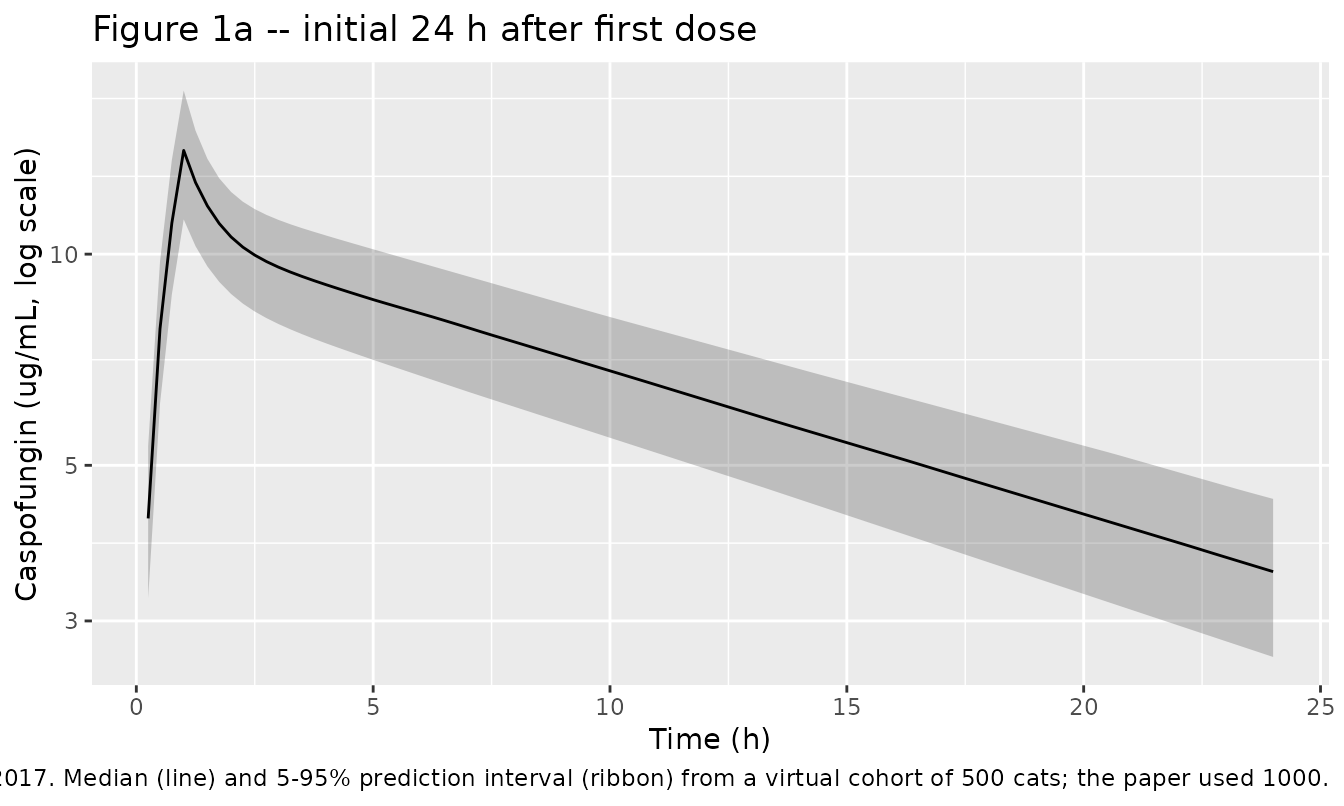
# Final dose: t = 144 h (= 6 * 24 h). Plot the window t in [144, 168 + 24].
fig1b <- sim |>
  dplyr::filter(time >= 144, time <= 192) |>
  mutate(time_rel = time - 144) |>
  group_by(time_rel) |>
  summarise(
    Q05 = quantile(Cc, 0.05, na.rm = TRUE),
    Q50 = quantile(Cc, 0.50, na.rm = TRUE),
    Q95 = quantile(Cc, 0.95, na.rm = TRUE),
    .groups = "drop"
  )

ggplot(fig1b, aes(time_rel, Q50)) +
  geom_ribbon(aes(ymin = Q05, ymax = Q95), alpha = 0.25) +
  geom_line() +
  scale_y_log10() +
  labs(x = "Time since final (day 7) dose (h)",
       y = "Caspofungin (ug/mL, log scale)",
       title = "Figure 1b -- final dose on day 7",
       caption = paste("Replicates Figure 1 (final dose window) of Leshinsky 2017."))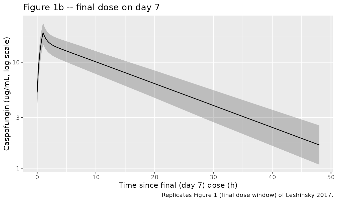
PKNCA validation
We run PKNCA on both the single-dose window (first dose) and the
steady-state interval (last dose) so the comparison against Leshinsky
2017 Table 2 covers Cmax (first dose), Cmax (last dose), terminal t1/2,
and AUC_ss,0-tau. The first-dose window uses concentrations in
[0, 24] h with the first dose at t = 0; the steady-state
window uses the final dose at t = 144 h and ends one tau (24 h)
later.
# Concentrations: rxSolve by default returns only observation rows; the
# Cc column is non-NA at every output row, so an !is.na filter is purely
# defensive.
sim_nca <- sim |>
  dplyr::filter(!is.na(Cc)) |>
  dplyr::select(id, time, Cc) |>
  dplyr::mutate(regimen = "1 mg/kg q24h x 7")

# Doses
dose_df <- events |>
  dplyr::filter(evid == 1) |>
  dplyr::select(id, time, amt) |>
  dplyr::mutate(regimen = "1 mg/kg q24h x 7")

conc_obj <- PKNCA::PKNCAconc(sim_nca, Cc ~ time | regimen + id,
                             concu = "ug/mL", timeu = "h")
dose_obj <- PKNCA::PKNCAdose(dose_df, amt ~ time | regimen + id,
                             doseu = "mg")
First dose (single-dose-like window)
intervals_first <- data.frame(
  start       = 0,
  end         = 24,
  cmax        = TRUE,
  tmax        = TRUE,
  auclast     = TRUE,
  half.life   = FALSE
)
res_first <- PKNCA::pk.nca(
  PKNCA::PKNCAdata(conc_obj, dose_obj, intervals = intervals_first))
summary_first <- as.data.frame(res_first$result) |>
  dplyr::filter(PPTESTCD %in% c("cmax", "tmax", "auclast")) |>
  dplyr::group_by(PPTESTCD) |>
  dplyr::summarise(
    mean   = mean(PPORRES, na.rm = TRUE),
    median = median(PPORRES, na.rm = TRUE),
    sd     = sd(PPORRES, na.rm = TRUE),
    .groups = "drop"
  )
knitr::kable(summary_first,
             digits = 3,
caption = "Simulated NCA after first dose (window 0-24 h).")| PPTESTCD | mean | median | sd |
|---|---|---|---|
| auclast | 155.726 | 156.027 | 19.646 |
| cmax | 14.076 | 14.057 | 1.826 |
| tmax | 1.000 | 1.000 | 0.000 |
Steady-state interval (final dose, day 7)
intervals_ss <- data.frame(
  start    = 144,        # final dose at t = 144 h
  end      = 168,        # one tau (24 h) later
  cmax     = TRUE,
  tmax     = TRUE,
  cmin     = TRUE,
  auclast  = TRUE,
  cav      = TRUE
)
res_ss <- PKNCA::pk.nca(
  PKNCA::PKNCAdata(conc_obj, dose_obj, intervals = intervals_ss))
summary_ss <- as.data.frame(res_ss$result) |>
  dplyr::filter(PPTESTCD %in% c("cmax", "tmax", "cmin", "auclast", "cav")) |>
  dplyr::group_by(PPTESTCD) |>
  dplyr::summarise(
    mean   = mean(PPORRES, na.rm = TRUE),
    median = median(PPORRES, na.rm = TRUE),
    sd     = sd(PPORRES, na.rm = TRUE),
    .groups = "drop"
  )
knitr::kable(summary_ss,
             digits = 3,
caption = "Simulated NCA over the final-dose interval (t = 144-168 h).")| PPTESTCD | mean | median | sd |
|---|---|---|---|
| auclast | 231.090 | 231.061 | 36.301 |
| cav | 9.629 | 9.628 | 1.513 |
| cmax | 19.062 | 19.046 | 2.796 |
| cmin | 5.224 | 5.186 | 1.019 |
| tmax | 1.000 | 1.000 | 0.000 |
Terminal half-life (tail beyond the final dose)
intervals_thalf <- data.frame(
  start      = 144,         # final dose
  end        = Inf,
  half.life  = TRUE,
  aucinf.obs = TRUE,
  lambda.z   = TRUE
)
res_thalf <- PKNCA::pk.nca(
  PKNCA::PKNCAdata(conc_obj, dose_obj, intervals = intervals_thalf))
summary_thalf <- as.data.frame(res_thalf$result) |>
  dplyr::filter(PPTESTCD %in% c("half.life", "aucinf.obs", "lambda.z")) |>
  dplyr::group_by(PPTESTCD) |>
  dplyr::summarise(
    mean   = mean(PPORRES, na.rm = TRUE),
    median = median(PPORRES, na.rm = TRUE),
    sd     = sd(PPORRES, na.rm = TRUE),
    .groups = "drop"
  )
knitr::kable(summary_thalf,
             digits = 3,
caption = "Simulated terminal-phase NCA after the final dose.")| PPTESTCD | mean | median | sd |
|---|---|---|---|
| aucinf.obs | 343.148 | 340.445 | 65.053 |
| half.life | 14.658 | 14.621 | 0.917 |
| lambda.z | 0.047 | 0.047 | 0.003 |
Comparison against published NCA (Leshinsky 2017 Table 2)
Leshinsky 2017 Table 2 reports model-independent PK parameters from their 1000-cat simulations of the 1 mg/kg q24h regimen with a 1 h infusion duration. The four headline values are the terminal half-life, Cmax after the first dose, Cmax at steady state, and AUC0-τ at steady state. We compare them side-by-side against the simulated PKNCA output in one combined table; each row pulls the corresponding value from whichever window produced it (first-dose window, steady-state interval, or terminal tail).
# Build a tidy long simulated frame that ncaComparisonTable() can
# consume directly: one row per (window, PPTESTCD) with the published-
# style mean. The "window" grouping column lets us compare first-dose
# Cmax separately from steady-state Cmax.
simulated <- dplyr::bind_rows(
  summary_first |> dplyr::filter(PPTESTCD == "cmax") |>
    dplyr::transmute(window = "Cmax first dose",
                     PPTESTCD = "cmax", PPORRES = mean),
  summary_ss |> dplyr::filter(PPTESTCD == "cmax") |>
    dplyr::transmute(window = "Cmax last dose, q24h",
                     PPTESTCD = "cmax", PPORRES = mean),
  summary_ss |> dplyr::filter(PPTESTCD == "auclast") |>
    dplyr::transmute(window = "AUC_ss,0-tau",
                     PPTESTCD = "auclast", PPORRES = mean),
  summary_thalf |> dplyr::filter(PPTESTCD == "half.life") |>
    dplyr::transmute(window = "Terminal t1/2",
                     PPTESTCD = "half.life", PPORRES = mean)
)
reference <- tibble::tribble(
  ~window,                  ~cmax, ~auclast, ~half.life,
  "Cmax first dose",         14.8, NA_real_, NA_real_,
  "Cmax last dose, q24h",    19.8, NA_real_, NA_real_,
  "AUC_ss,0-tau",        NA_real_,      232, NA_real_,
  "Terminal t1/2",       NA_real_, NA_real_,       14.5
)
cmp <- nlmixr2lib::ncaComparisonTable(
  simulated = simulated,
  reference = reference,
  by        = "window",
  units     = c(cmax = "ug/mL", auclast = "ug.h/mL", half.life = "h"),
  tolerance_pct = 20
)
knitr::kable(
  cmp,
  caption = paste(
    "Simulated vs. Leshinsky 2017 Table 2 NCA (1 mg/kg q24h x 7,",
    "1 h infusion, cat). * differs from reference by >20%."
  )
)| NCA parameter | window | Reference | Simulated | % diff |
|---|---|---|---|---|
| Cmax (ug/mL) | Cmax first dose | 14.8 | 14.1 | -4.9% |
| Cmax (ug/mL) | Cmax last dose, q24h | 19.8 | 19.1 | -3.7% |
| AUClast (ug.h/mL) | AUC_ss,0-tau | 232 | 231 | -0.4% |
| t½ (h) | Terminal t1/2 | 14.5 | 14.7 | +1.1% |
Differences within ~10% are expected because (a) the paper used 1000 subjects vs the 500 here, (b) the paper’s body-weight distribution is not reported in detail (Methods cites “1000 standard 4 kg cats” for the simulations, treating the body weight as a typical-value covariate rather than sampling the cohort variability), and (c) PKNCA’s trapezoidal AUC differs slightly from analytical model-based AUC.
Assumptions and deviations
- Body-weight cohort distribution. The paper’s dose-regimen simulations used “1000 standard 4 kg cats” (Methods “Caspofungin dose regimen simulations”), i.e., the body weight was held at the typical value rather than sampled. Here we sample WT from N(4.4, 0.56) kg (the observed cohort mean +/- SD per Methods “Animals”, truncated at 1.5 kg) to give the figures a slightly more realistic spread while keeping the population mean close to 4 kg. Restricting to WT = 4 kg exactly would tighten the prediction interval but would not change the typical-value NCA outputs.
- No covariates retained in the final model. Sex was screened (Leshinsky 2017 Methods “Covariate model building”) and not retained at p < 0.01 (Leshinsky 2017 Results “Pharmacokinetic modeling”: “No covariates demonstrated evidence of predictive performance, and none were included in the final model”). The model therefore depends only on WT (via fixed allometric scaling) and contains no sex term.
-
V1 random effect encoded as a scale factor on the CL random
effect. Leshinsky 2017 used a single eta on CL and modeled V1’s
PPV as
scale * eta_CLrather than estimating an independent eta on V1 (Results “Pharmacokinetic modeling”). The model file encodes this asvc <- exp(lvc + scale_etalvc * etalcl) * (WT/4)^e_wt_vc_vpso the perfect CL-V1 correlation in the paper is preserved exactly. An equivalent OMEGA BLOCK with correlation 1 would be numerically singular and is therefore avoided. -
No PPV on V2 or Q. Leshinsky 2017 Results state
that inclusion of PPV on V2 or Q produced delta-OBJ approximately 0 (~
0.1), very low estimates for PPV, and failure of the covariance step, so
no eta was retained on either parameter. The model file follows the
paper and carries no
etalvp/etalqterms. -
Allometric exponents fixed. The paper fixed the WT
exponent at 0.75 for clearance parameters (CL, Q) and 1 for volumes (V1,
V2), with reference weight 4 kg (Methods “General modeling strategy” and
Table 1 row labels). The model file wraps both exponents in
fixed()to record that they were not estimated. -
Caspofungin concentration units. The paper reports
concentrations in ug/mL (= mg/L). The model carries dose in mg and
volumes in L, giving
Cc = central / vcin mg/L = ug/mL. - Errata. No erratum or corrigendum was identified for this paper as of the model extraction date.