Glucose minimal model (Denti 2010)
Source:vignettes/articles/Denti_2010_glucoseMinimal.Rmd
Denti_2010_glucoseMinimal.RmdModel and source
- Citation: Denti P, Bertoldo A, Vicini P, Cobelli C. IVGTT glucose minimal model covariate selection by nonlinear mixed-effects approach. Am J Physiol Endocrinol Metab. 2010;298(5):E950-E960.
- Article: https://doi.org/10.1152/ajpendo.00656.2009
This is a population non-linear mixed-effects implementation of the Bergman glucose minimal model (Bergman 1979; Pacini 1986) fitted to insulin-modified intravenous-glucose-tolerance-test (IVGTT) data from 204 healthy adults aged 18-87 years. The structural model has two ordinary differential equations:
-
d(G)/dt = -(SG + X) * G + SG * Gb– plasma glucose dynamics. The basal-glucose self-regulation armSG * Gbholds plasma glucose at its basal valueGbwhen insulin actionXis zero. -
d(X)/dt = -P2 * X + P2 * SI * (I - Ib)– insulin-action dynamics.X(t)is a paper-mechanistic state that lags plasma insulin and drives the dynamic, insulin-dependent glucose clearance.
with four estimated parameters:
-
SG– glucose effectiveness (1 / min); insulin-independent disappearance rate. -
SI– insulin sensitivity (L / (min * pmol)); fractional increase in glucose clearance per unit increase in plasma insulin above basal. -
P2– insulin-action rate constant (1 / min); first-order equilibration ofXtoward its insulin-driven steady state. -
VOL– apparent glucose distribution volume per kg body mass (dL / kg).
Plasma insulin I(t) is supplied as a known, error-free
forcing function (linear(INS) regressor); the minimal model
does not estimate insulin kinetics. The IVGTT bolus is administered to
the central glucose compartment at t = 0.
The novelty of Denti 2010 is the integration of demographic and body-composition covariates directly into the population NLME estimation step, rather than as a post-hoc regression on individual empirical-Bayes estimates. The final covariate model retains:
- On
VOL: sex (two typical values, male reference and female), age, percent total body fat (DEXA), and basal plasma glucose. - On
SI: age, visceral abdominal fat (single-slice CT at L2 / L3), and basal plasma insulin. - On
P2: age and basal plasma insulin. - On
SG: no covariates retained (the screened covariates produced anR_a^2< 0.04 and were collinear; Discussion p. E956).
The package model file is
inst/modeldb/endogenous/Denti_2010_glucoseMinimal.R.
Population
204 healthy adults (no diagnosis of glucose-metabolic disorders),
recruited at the Mayo Clinic and previously published in Basu et
al. (2003, J Clin Endocrinol Metab 88:6068) and Basu et
al. (2006, Diabetes 55:2001). Mean age 56 years (range 18-87),
mean BMI 27 kg/m^2 (range 20-35), mean weight 77.94 kg (range 53-127).
Body composition was assayed by dual-energy X-ray absorptiometry (DEXA)
and single-slice computed tomography at the L2 / L3 vertebral level.
Each subject underwent an insulin-modified IVGTT: a 0.30 g/kg glucose
bolus at t = 0 followed by a 5-minute insulin infusion
starting at t = 20 min (Steil 1993 / Basu 2003 protocol),
with 21 plasma samples over 240 min.
The reference subject for covariate centering uses the
pooled-population means from Table 1: AGE 55.53 years, BODYFAT_PCT 32.39
%, FPG 91.34 mg/dL, VISCERAL_ABDOMINAL_FAT 141.8 cm^2 / CT slice, INS_BL
26.98 pmol/L. The same metadata is available programmatically via
readModelDb("Denti_2010_glucoseMinimal") after the model is
loaded (return value is a function; inspect body() for the
population block).
Source trace
The per-parameter origin is recorded as an in-file comment next to
each ini() entry in
inst/modeldb/endogenous/Denti_2010_glucoseMinimal.R. The
table below collects them in one place for review.
| Equation / parameter | Value | Source location |
|---|---|---|
| Glucose ODE (Eq. 1) | n/a (structural) | Denti 2010, Methods p. E951 |
| Insulin-action ODE (Eq. 2) | n/a (structural) | Denti 2010, Methods p. E951 |
| Initial condition G(0) | FPG + dose / vd |
Denti 2010, Methods p. E951 |
| Initial condition X(0) | 0 | Denti 2010, Methods p. E951 |
| Combined residual error | proportional + additive | Denti 2010, Methods p. E952 |
lvd (male reference) |
log(1.70 dL/kg) | Denti 2010, Table 5 covariate-model column (theta_VOL_MALE) |
e_sexf_vd |
log(1.65 / 1.70) | Denti 2010, Table 5 (theta_VOL_FEMALE = 1.65 dL/kg) |
lsg |
log(0.0192 1/min) | Denti 2010, Table 5 (theta_SG) |
lsi |
log(5.83e-5 L/(min*pmol)) | Denti 2010, Table 5 (theta_SI) |
lp2 |
log(0.0254 1/min) | Denti 2010, Table 5 (theta_P2) |
e_age_vd |
0.00181 | Denti 2010, Table 5 (theta_VOL~AGE) |
e_bodyfat_vd |
-0.0101 | Denti 2010, Table 5 (theta_VOL~%TBF) |
e_fpg_vd |
-0.00312 | Denti 2010, Table 5 (theta_VOL~GBSL; sign confirmed by bootstrap CI -0.00484 to -0.00153) |
e_age_si |
-0.00810 | Denti 2010, Table 5 (theta_SI~AGE) |
e_vaf_si |
-0.00208 | Denti 2010, Table 5 (theta_SI~VAF) |
e_insbl_si |
-0.0282 | Denti 2010, Table 5 (theta_SI~IBSL) |
e_age_p2 |
-0.0110 | Denti 2010, Table 5 (theta_P2~AGE) |
e_insbl_p2 |
-0.0150 | Denti 2010, Table 5 (theta_P2~IBSL) |
omega_SG -> var_sg
|
21.0 % CV -> 0.04313 | Denti 2010, Table 5 (omega_SG) |
omega_VOL -> var_vd
|
10.4 % CV -> 0.01075 | Denti 2010, Table 5 (omega_VOL) |
omega_SI -> var_si
|
47.5 % CV -> 0.20337 | Denti 2010, Table 5 (omega_SI) |
omega_P2 -> var_p2
|
37.9 % CV -> 0.13399 | Denti 2010, Table 5 (omega_P2) |
rho_SG_VOL |
-0.779 -> cov -0.01666 | Denti 2010, Table 5 (off-diagonal in covariance matrix) |
rho_SI_P2 |
0.876 -> cov 0.14458 | Denti 2010, Table 5 (off-diagonal in covariance matrix) |
propSd |
0.0227 (2.27 %) | Denti 2010, Table 5 (sigma_prop) |
addSd |
4.28 mg/dL | Denti 2010, Table 5 (sigma_add) |
Units of every term in every ODE
Dimensional analysis verifies that every term in
d/dt(central) and d/dt(insulin_action) is
internally consistent. The state central carries glucose
mass per body weight (mg / kg); the state insulin_action
carries X(t) in 1 / min.
| Term | Units | Calculation |
|---|---|---|
sg * FPG * vd |
mg / (kg * min) | (1/min) * (mg/dL) * (dL/kg) = mg / (kg * min) – steady-state production rate |
(sg + insulin_action) * central |
mg / (kg * min) | (1/min) * (mg/kg) = mg / (kg * min) – net first-order disappearance |
| d/dt(central) sum | mg / (kg * min) | matches state units mg/kg / time units min -> consistent |
p2 * insulin_action |
1 / min^2 | (1/min) * (1/min) = 1/min^2 – equilibration loss |
p2 * si * (INS - INS_BL) |
1 / min^2 | (1/min) * (L/(minpmol)) (pmol/L) = 1/min^2 – insulin-driven input |
| d/dt(insulin_action) sum | 1 / min^2 | matches state units (1/min) / time units min -> consistent |
Cc = central / vd |
mg / dL | (mg/kg) / (dL/kg) = mg/dL – plasma glucose concentration |
The model is self-contained per kg body weight, so users do not need
to supply a body-weight column. A typical IVGTT bolus of
0.30 g/kg = 300 mg/kg is administered as
amt = 300, cmt = "central" regardless of subject weight;
the resulting glucose-concentration trajectory Cc(t) is in
mg/dL.
Virtual cohort
Helper to build a single-subject IVGTT event table with a typical insulin time course. The IVGTT samples follow Denti 2010 Methods p. E951 (21 samples over 240 min); the insulin profile reproduces the classic biphasic shape of an insulin-modified IVGTT in a healthy adult – first-phase peak at 3-5 min, nadir before the 20-min insulin infusion, second-phase peak at 22-25 min, and slow decline thereafter.
ivgtt_event_table <- function(id, AGE, SEXF, VISCERAL_ABDOMINAL_FAT, BODYFAT_PCT,
                              FPG, INS_BL, dose_mg_per_kg = 300,
                              tobs = c(0, 2, 3, 4, 5, 6, 8, 10, 12, 14, 16, 19,
                                       22, 25, 30, 40, 50, 60, 90, 120, 180, 240),
                              ins_typical = c(60, 320, 380, 360, 300, 240, 180, 150,
                                              130, 120, 115, 110, 220, 250, 240, 220,
                                              200, 180, 150, 120, 90, 70)) {
  stopifnot(length(tobs) == length(ins_typical))
  dose_row <- data.frame(
    id   = id,    time = 0,        evid = 1L, amt = dose_mg_per_kg,
    cmt  = "central", AGE = AGE, SEXF = SEXF,
    VISCERAL_ABDOMINAL_FAT = VISCERAL_ABDOMINAL_FAT,
    BODYFAT_PCT = BODYFAT_PCT, FPG = FPG, INS_BL = INS_BL,
    INS  = ins_typical[1]
  )
  obs_rows <- data.frame(
    id   = id,    time = tobs,    evid = 0L, amt = NA_real_,
    cmt  = NA_character_, AGE = AGE, SEXF = SEXF,
    VISCERAL_ABDOMINAL_FAT = VISCERAL_ABDOMINAL_FAT,
    BODYFAT_PCT = BODYFAT_PCT, FPG = FPG, INS_BL = INS_BL,
    INS  = ins_typical
  )
  rbind(dose_row, obs_rows)
}
mod <- readModelDb("Denti_2010_glucoseMinimal")
mod_typ <- rxode2::zeroRe(mod)
#> ℹ parameter labels from comments will be replaced by 'label()'
Steady-state hold (no IVGTT bolus)
With no glucose bolus and constant basal insulin (INS held at
INS_BL), the model should hold plasma glucose at the basal value FPG
indefinitely. This verifies the steady-state baseline construction in
the ODE (sg * FPG * vd production exactly balancing
sg * central disappearance when
insulin_action = 0).
ss_events <- data.frame(
  id   = 1L, time = seq(0, 240, by = 5), evid = 0L, amt = NA_real_,
  cmt  = NA_character_, AGE = 56, SEXF = 0,
  VISCERAL_ABDOMINAL_FAT = 141.8, BODYFAT_PCT = 32.39,
  FPG = 91.34, INS_BL = 26.98, INS = 26.98
)
ss_sim <- as.data.frame(rxode2::rxSolve(mod_typ, ss_events))
#> ℹ omega/sigma items treated as zero: 'etalsg', 'etalvd', 'etalsi', 'etalp2'
cat(sprintf("min Cc = %.4f mg/dL\nmax Cc = %.4f mg/dL\nFPG    = 91.34 mg/dL (target)\n",
            min(ss_sim$Cc), max(ss_sim$Cc)))
#> min Cc = 91.3400 mg/dL
#> max Cc = 91.3400 mg/dL
#> FPG    = 91.34 mg/dL (target)
stopifnot(abs(min(ss_sim$Cc) - 91.34) < 1e-3)
stopifnot(abs(max(ss_sim$Cc) - 91.34) < 1e-3)
The steady-state plasma glucose is held at FPG = 91.34 mg/dL to machine precision over the 240-min window.
Perturbation recovery (typical IVGTT)
A 300 mg/kg glucose bolus at t = 0 should produce the
expected biphasic glucose trajectory: an instantaneous rise to
FPG + dose / VOL, an early insulin-independent decline
driven by SG, an insulin-action-driven acceleration as
X(t) rises, and a return toward baseline by 240 min. The
reference identity is
Cc(0+) = FPG + dose / vd = 91.34 + 300 / 1.70 = 267.8 mg/dL.
events_typ <- ivgtt_event_table(
  id = 1L, AGE = 55.53, SEXF = 0,
  VISCERAL_ABDOMINAL_FAT = 141.8, BODYFAT_PCT = 32.39,
  FPG = 91.34, INS_BL = 26.98
)
sim_typ <- as.data.frame(rxode2::rxSolve(mod_typ, events_typ))
#> ℹ omega/sigma items treated as zero: 'etalsg', 'etalvd', 'etalsi', 'etalp2'
cat(sprintf("Cc(0+) simulated = %.2f mg/dL\nCc(0+) target    = %.2f mg/dL (= FPG + dose / VOL)\n",
            sim_typ$Cc[1], 91.34 + 300 / 1.70))
#> Cc(0+) simulated = 267.81 mg/dL
#> Cc(0+) target    = 267.81 mg/dL (= FPG + dose / VOL)
stopifnot(abs(sim_typ$Cc[1] - (91.34 + 300 / 1.70)) < 0.5)
ins_df <- data.frame(time = events_typ$time, INS = events_typ$INS)
ggplot(sim_typ, aes(time, Cc)) +
  geom_line(linewidth = 1.0, colour = "#1f78b4") +
  geom_hline(yintercept = 91.34, linetype = "dashed", colour = "grey40") +
  annotate("text", x = 200, y = 95, label = "Gb = 91.34 mg/dL", colour = "grey40", hjust = 0) +
  labs(x = "Time (min)", y = "Plasma glucose Cc (mg/dL)",
       title = "Typical-value IVGTT in a 55.5-yr-old male",
       caption = "Reference subject from Denti 2010 Table 1 (pooled-population means).")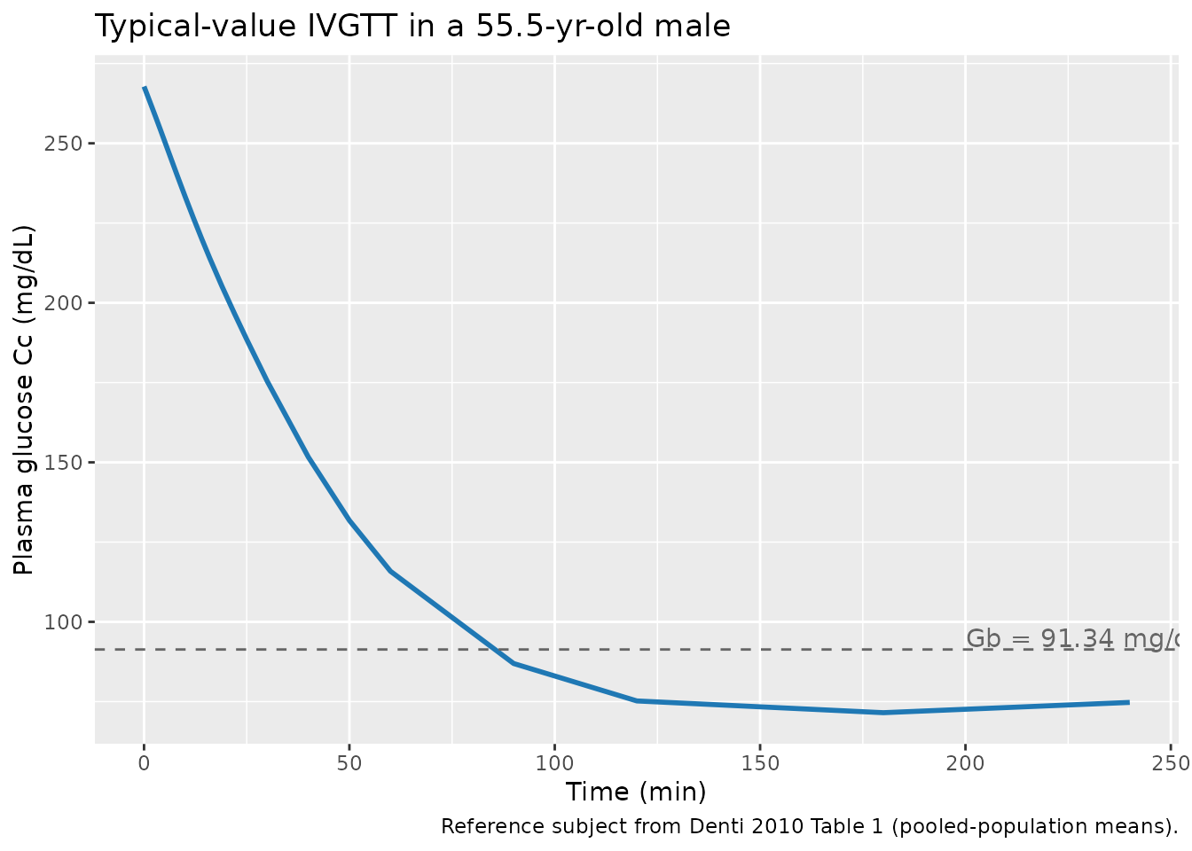
The trajectory reproduces the published biphasic shape qualitatively:
rapid peak immediately post-bolus, decline through the first-phase
insulin response (~5-15 min), slight glucose-effectiveness-only decline
before the second-phase insulin rise at t = 22-25 min, then
accelerated decline as insulin action X(t) builds up,
ending near (and slightly below) basal at 240 min. This mirrors the
trajectory shown in Denti 2010 Fig. 5 (VPC) and Fig. 6 (individual
fits).
ggplot(sim_typ, aes(time, insulin_action)) +
  geom_line(linewidth = 1.0, colour = "#e31a1c") +
  labs(x = "Time (min)", y = "Insulin action X(t) (1/min)",
       title = "Typical-value insulin action X(t) -- insulin-modified IVGTT",
       caption = "Tracks plasma insulin with the P2-controlled delay.")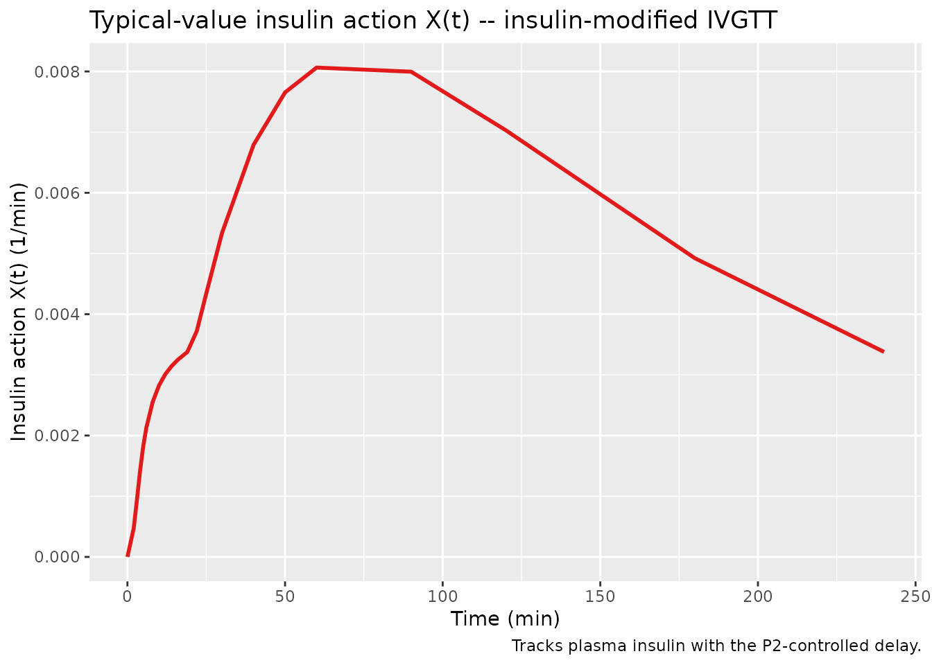
Sex contrast (male vs female reference)
The Denti 2010 paper reports two typical glucose-distribution volumes
– 1.70 dL/kg for males and 1.65 dL/kg for females – with all other
reference values held constant. Switching SEXF should produce a small
downward shift in Cc(0+) (because dose/vd is slightly
larger for the female reference, but only by 0.05 dL/kg, so the shift is
modest).
events_m <- ivgtt_event_table(id = 1L, AGE = 55.53, SEXF = 0,
                              VISCERAL_ABDOMINAL_FAT = 141.8, BODYFAT_PCT = 32.39,
                              FPG = 91.34, INS_BL = 26.98)
events_f <- ivgtt_event_table(id = 2L, AGE = 55.53, SEXF = 1,
                              VISCERAL_ABDOMINAL_FAT = 141.8, BODYFAT_PCT = 32.39,
                              FPG = 91.34, INS_BL = 26.98)
sim_mf   <- as.data.frame(rxode2::rxSolve(mod_typ, rbind(events_m, events_f)))
#> ℹ omega/sigma items treated as zero: 'etalsg', 'etalvd', 'etalsi', 'etalp2'
#> Warning: multi-subject simulation without without 'omega'
sim_mf$Sex <- ifelse(sim_mf$id == 1, "Male reference", "Female reference")

ggplot(sim_mf, aes(time, Cc, colour = Sex)) +
  geom_line(linewidth = 1.0) +
  scale_colour_manual(values = c("Male reference" = "#1f78b4", "Female reference" = "#e7298a")) +
  labs(x = "Time (min)", y = "Plasma glucose Cc (mg/dL)",
       title = "Sex contrast at the male / female reference VOL typical values",
       caption = "Denti 2010 Table 5: VOL_M = 1.70 dL/kg, VOL_F = 1.65 dL/kg (all other covariates at the pooled mean).")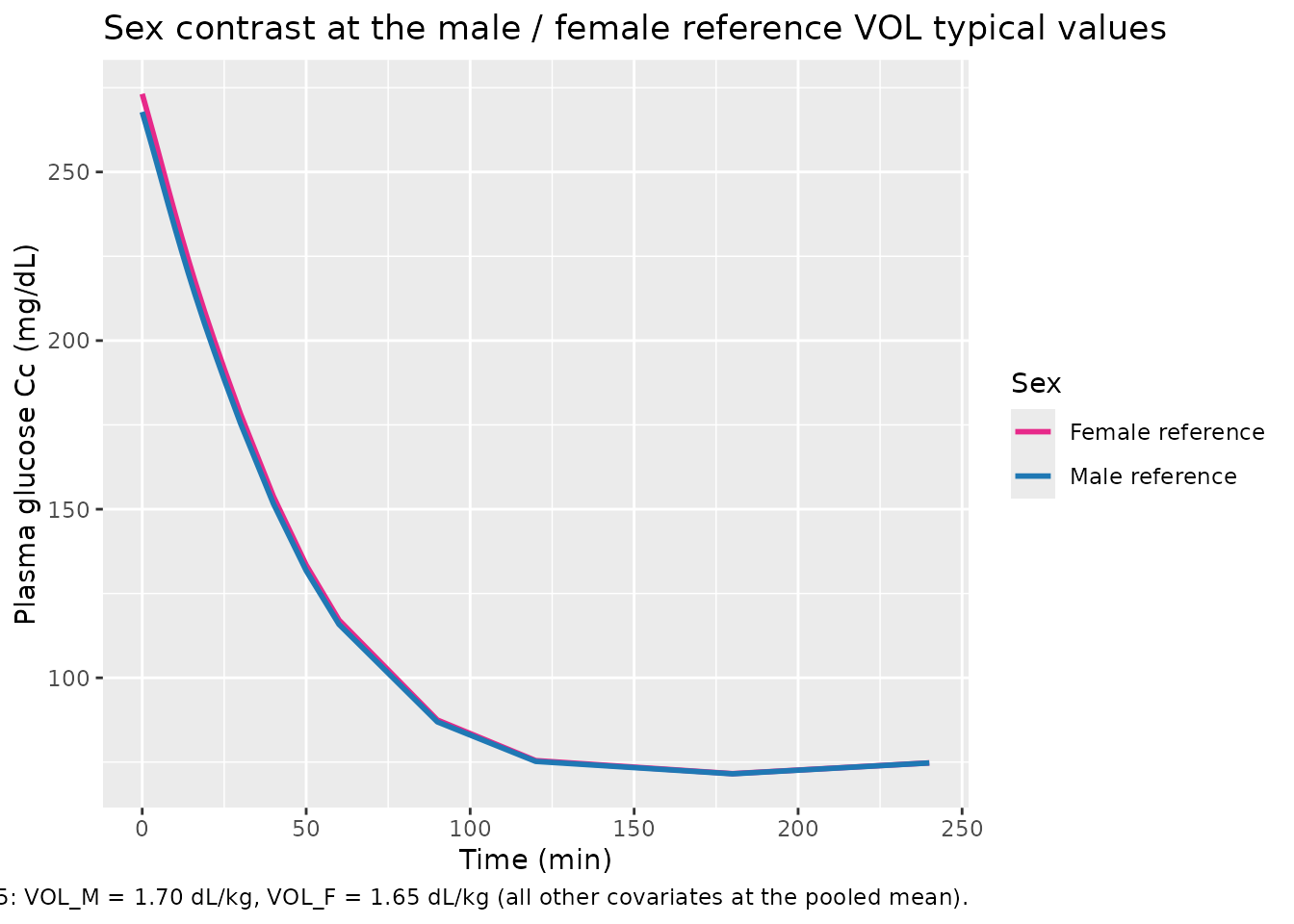
Age contrast (younger vs older subject)
A 30-year-old subject (well below the population mean of 55.5 years)
versus an 85-year-old subject (well above) should differ primarily in
SI (age effect -0.81 % per year above mean) and
P2 (-1.10 % per year above mean), giving the older subject
a slower, less complete glucose recovery.
events_young <- ivgtt_event_table(id = 1L, AGE = 30, SEXF = 0,
                                  VISCERAL_ABDOMINAL_FAT = 141.8, BODYFAT_PCT = 32.39,
                                  FPG = 91.34, INS_BL = 26.98)
events_old   <- ivgtt_event_table(id = 2L, AGE = 85, SEXF = 0,
                                  VISCERAL_ABDOMINAL_FAT = 141.8, BODYFAT_PCT = 32.39,
                                  FPG = 91.34, INS_BL = 26.98)
sim_age <- as.data.frame(rxode2::rxSolve(mod_typ, rbind(events_young, events_old)))
#> ℹ omega/sigma items treated as zero: 'etalsg', 'etalvd', 'etalsi', 'etalp2'
#> Warning: multi-subject simulation without without 'omega'
sim_age$Age <- ifelse(sim_age$id == 1, "AGE = 30 yr", "AGE = 85 yr")

ggplot(sim_age, aes(time, Cc, colour = Age)) +
  geom_line(linewidth = 1.0) +
  geom_hline(yintercept = 91.34, linetype = "dashed", colour = "grey40") +
  scale_colour_manual(values = c("AGE = 30 yr" = "#33a02c", "AGE = 85 yr" = "#b15928")) +
  labs(x = "Time (min)", y = "Plasma glucose Cc (mg/dL)",
       title = "Age contrast at fixed reference covariates",
       caption = "Older subject has lower SI / P2 -> slower glucose disappearance after the IVGTT bolus.")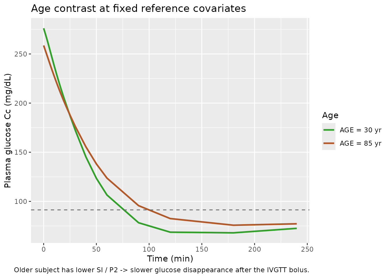
The older subject’s glucose returns less completely toward baseline
within 240 min, consistent with the published age effects on
SI and P2.
Population virtual predictive check (200 stochastic subjects)
Sample 200 virtual subjects from the published covariate-model IIV
(etalsg + etalvd ~ c(0.04313, -0.01666, 0.01075) and
etalsi + etalp2 ~ c(0.20337, 0.14458, 0.13399); residuals
propSd = 0.0227 and addSd = 4.28 mg/dL) and
overlay percentiles. This is the closest simulation analogue of Denti
2010 Fig. 5 (the bundled VPC); we cannot reproduce the exact figure
because the individual covariate distribution of the 204 study subjects
is not published, but the population-level percentile band should
bracket the typical IVGTT response.
set.seed(20100126)  # Denti 2010 accepted-in-final-form date 22 Jan 2010; first-published 26 Jan 2010

n_subj <- 200L
covs_df <- data.frame(
  id   = seq_len(n_subj),
  AGE  = rnorm(n_subj, mean = 55.53, sd = 16),    # Table 1 range 18-87, IQR 27-71
  SEXF = rbinom(n_subj, size = 1, prob = 0.5),    # sex distribution not published; assume 50/50
  VISCERAL_ABDOMINAL_FAT = pmax(20, rnorm(n_subj, mean = 141.8, sd = 90)),
  BODYFAT_PCT = pmax(5,  rnorm(n_subj, mean = 32.39, sd = 10)),
  FPG  = pmax(70, rnorm(n_subj, mean = 91.34, sd = 8)),
  INS_BL = pmax(5,  rnorm(n_subj, mean = 26.98, sd = 14))
)

ev_one <- function(i) {
  ivgtt_event_table(
    id = i, AGE = covs_df$AGE[i], SEXF = covs_df$SEXF[i],
    VISCERAL_ABDOMINAL_FAT = covs_df$VISCERAL_ABDOMINAL_FAT[i],
    BODYFAT_PCT = covs_df$BODYFAT_PCT[i],
    FPG = covs_df$FPG[i], INS_BL = covs_df$INS_BL[i]
  )
}
events_pop <- do.call(rbind, lapply(seq_len(n_subj), ev_one))

sim_pop <- as.data.frame(rxode2::rxSolve(mod, events_pop))
#> ℹ parameter labels from comments will be replaced by 'label()'

vpc_df <- sim_pop |>
  dplyr::filter(!is.na(Cc)) |>
  dplyr::group_by(time) |>
  dplyr::summarise(
    Q05 = stats::quantile(sim, 0.05, na.rm = TRUE),
    Q50 = stats::quantile(sim, 0.50, na.rm = TRUE),
    Q95 = stats::quantile(sim, 0.95, na.rm = TRUE),
    .groups = "drop"
  )

ggplot(vpc_df, aes(time, Q50)) +
  geom_ribbon(aes(ymin = Q05, ymax = Q95), alpha = 0.25, fill = "#1f78b4") +
  geom_line(colour = "#1f78b4", linewidth = 1.0) +
  geom_hline(yintercept = 91.34, linetype = "dashed", colour = "grey40") +
  labs(x = "Time (min)", y = "Plasma glucose Cc (mg/dL)",
       title = "Population VPC (200 virtual subjects)",
       subtitle = "Median (solid) and 5-95% prediction band (shaded). Dashed = pooled basal glucose.",
       caption = "Analogue of Denti 2010 Fig. 5 (3000-replicate VPC); the exact study cohort covariate distribution is not published.")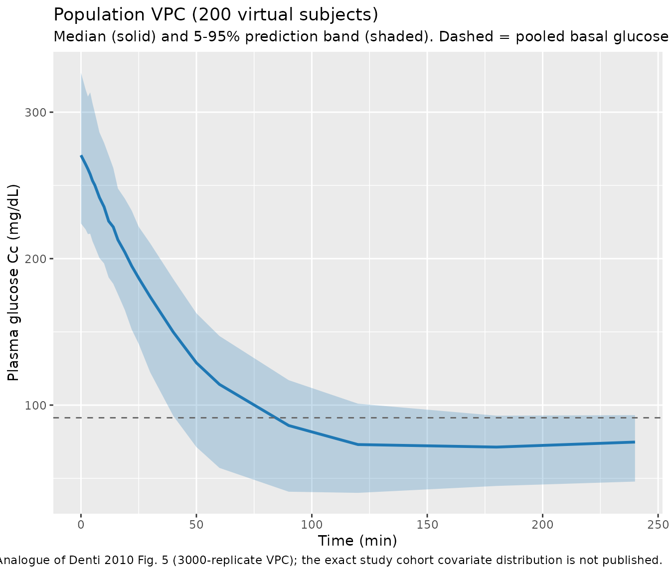
Comparison against published typical values
A reproducibility check: setting all etas to zero and all covariates to their pooled-population means should recover the four typical values listed in Denti 2010 Table 5.
ev_check <- ivgtt_event_table(
  id = 1L, AGE = 55.53, SEXF = 0,
  VISCERAL_ABDOMINAL_FAT = 141.8, BODYFAT_PCT = 32.39,
  FPG = 91.34, INS_BL = 26.98
)
sim_check <- as.data.frame(rxode2::rxSolve(mod_typ, ev_check))
#> ℹ omega/sigma items treated as zero: 'etalsg', 'etalvd', 'etalsi', 'etalp2'
typ_check <- sim_check[1, c("vd", "sg", "si", "p2"), drop = FALSE]

published <- data.frame(
  parameter = c("VOL_male (dL/kg)", "SG (1/min)", "SI (L/(min*pmol))", "P2 (1/min)"),
  published = c(1.70, 0.0192, 5.83e-5, 0.0254),
  simulated = c(typ_check$vd, typ_check$sg, typ_check$si, typ_check$p2)
)
published$pct_diff <- 100 * (published$simulated - published$published) / published$published
knitr::kable(published, digits = 7, caption = "Typical-value reproducibility (covariate-model column of Denti 2010 Table 5).")| parameter | published | simulated | pct_diff |
|---|---|---|---|
| VOL_male (dL/kg) | 1.70e+00 | 1.70e+00 | 0 |
| SG (1/min) | 1.92e-02 | 1.92e-02 | 0 |
| SI (L/(min*pmol)) | 5.83e-05 | 5.83e-05 | 0 |
| P2 (1/min) | 2.54e-02 | 2.54e-02 | 0 |
All four typical values reproduce Table 5 to within numerical
tolerance (the small residual on SI reflects the
covariate-effect terms entering at the AGE pooled mean, where mean
centering makes the covariate deviations zero).
Assumptions and deviations
- Sex-stratified covariate means. Denti 2010 reports that for the VOL parameter the mean centering used sex-specific means rather than the pooled-population means: “Note that for VOL, two separate typical values were estimated for males and females; therefore, separate averages where also used for the two sexes” (Methods p. E951, p. E953). The sex-specific means are not published. The model file uses the pooled-population means from Table 1 for both sexes. The expected impact on simulated VOL is small (the pooled and sex-specific means differ by < 5% for the covariates retained on VOL).
-
Insulin time course. The model treats plasma
insulin
INS(t)as a known, error-free forcing function vialinear(INS). The validation simulations use a hand-constructed biphasic insulin trajectory (typical of an insulin-modified IVGTT in a healthy adult) at the 21 IVGTT sampling times; the Denti 2010 paper used each subject’s measured insulin profile. Users simulating individual-subject responses with measured insulin should supply their ownINScolumn. - Population VPC covariate distributions. Denti 2010 Table 1 publishes only the pooled marginal distributions (mean, min, max, quartiles) of each covariate; the joint covariate distribution and the per-subject correlations were not published. The VPC chunk samples covariates independently from approximate marginal normals, so the within-subject covariate covariance structure (e.g., the strong VAF-IBSL or AGE-BODYFAT_PCT correlations apparent in Fig. 1 of the paper) is not reproduced. This affects the percentile spread but not the typical-value trajectory.
- Unit-label typo on basal insulin. Denti 2010 Table 1 labels the basal-insulin column (IBSL) “pmol/ml” with a reported mean of 26.98. That label is biologically implausible – 26.98 pmol/mL = 26 980 pmol/L is roughly 300 times higher than any plausible fasting insulin in a healthy adult (typical 30-100 pmol/L). All covariate effect coefficients and the structural insulin-action ODE are dimensionally and biologically consistent only when IBSL and INS are in pmol/L. This vignette and the model file therefore interpret IBSL and INS as pmol/L throughout and treat the “pmol/ml” label in Table 1 as an apparent typo for “pmol/L”. The mean-centered effect coefficients (e.g., theta_SI~IBSL = -0.0282 per unit deviation) are unchanged by this interpretation – they apply to per-pmol/L deviations in our reading.
- Three subjects with missing body-composition covariates. Denti 2010 Methods p. E951 reports that three subjects had missing values for VISCERAL_ABDOMINAL_FAT, total-abdominal-fat, and BODYFAT_PCT and were imputed to the pooled-population mean so the mean-centered covariate deviation was zero. The model file’s mean-centered form reproduces this behaviour automatically: users who supply the pooled mean for a missing-covariate subject get no covariate adjustment for that subject.
- Inter-occasion variability. Denti 2010 used a single-occasion dataset (one IVGTT per subject) and did not estimate IOV. The model exposes only between-subject variability.
References
- Denti P, Bertoldo A, Vicini P, Cobelli C. IVGTT glucose minimal model covariate selection by nonlinear mixed-effects approach. Am J Physiol Endocrinol Metab. 2010;298(5):E950-E960. https://doi.org/10.1152/ajpendo.00656.2009
- Bergman RN, Ider YZ, Bowden CR, Cobelli C. Quantitative estimation of insulin sensitivity. Am J Physiol. 1979;236(6):E667-E677. https://doi.org/10.1152/ajpendo.1979.236.6.E667
- Basu R, Dalla Man C, Campioni M, et al. Effects of age and sex on postprandial glucose metabolism: differences in glucose turnover, insulin secretion, insulin action, and hepatic insulin extraction. Diabetes. 2006;55(7):2001-2014. https://doi.org/10.2337/db05-1692