Enrofloxacin PD against Pasteurella multocida (Wen 2016)
Source:vignettes/articles/Wen_2016_enrofloxacin_Pmultocida.Rmd
Wen_2016_enrofloxacin_Pmultocida.RmdModel and source
- Citation: Wen X, Gehring R, Stallbaumer A, Riviere JE, Volkova VV. (2016). Limitations of MIC as sole metric of pharmacodynamic response across the range of antimicrobial susceptibilities within a single bacterial species. Scientific Reports 6:37907.
- Article: https://doi.org/10.1038/srep37907
This vignette validates the three packaged in-vitro pharmacodynamic
models (Wen_2016_enrofloxacin_MIC0p01,
Wen_2016_enrofloxacin_MIC1p5,
Wen_2016_enrofloxacin_MIC2p0) against the published Wen
2016 results. Because the model has no PK component (the drug
concentration is a static experimental input held constant in the broth)
and no fitted residual error on the bacterial density, PKNCA is not the
right validation target; the vignette instead reproduces the paper’s
published figures (time-kill trajectories from Figure 1,
parametric-uncertainty Monte-Carlo box-plots from Figures 2 and 3) and
checks the per-isolate concentration-effect curves against the
Discussion narrative.
Population
The paper used three Pasteurella multocida isolates from cattle respiratory organs (Methods, Bacterial isolates and antimicrobial agent paragraph):
-
Bovine lung (MIC = 0.01 ug/mL) – the
most-susceptible isolate. The Discussion describes this strain as
exhibiting the expected concentration-dependent enrofloxacin PD, with
EC50an order of magnitude higher than the MIC andEmaxof 1.64 log10(CFU/mL)/h. -
Bovine nasal swab (MIC = 1.5 ug/mL) – a
less-susceptible isolate exhibiting time-dependent PD characteristics.
EC50is close to the MIC andEmaxis roughly half the bovine-lung value. -
Bovine nasal swab (MIC = 2.0 ug/mL) – the
least-susceptible isolate with the steepest Hill coefficient (4.37) and
the lowest
Emax(0.69).
Susceptibility was determined by broth microdilution per the Clinical
and Laboratory Standards Institute (CLSI) protocol and confirmed by
E-test. All time-kill experiments used brain heart infusion (BHI) broth
at 37 C with shaking (200 rpm), a starting inoculum of 5 x 10^5 CFU/mL,
and a 24 h observation window with samples at 0, 1, 2, 3, 4, 5, 6, 7, 8,
12, and 24 h. For each isolate, seven enrofloxacin concentrations
corresponding to 0.5, 0.75, 1, 2, 3, 5, and 10 multiples of the
isolate’s MIC were studied, plus a no-drug control. The full per-isolate
metadata is accessible via
readModelDb(<model>)$population.
isolates <- c(
  low = "Wen_2016_enrofloxacin_MIC0p01",
  mid = "Wen_2016_enrofloxacin_MIC1p5",
  high = "Wen_2016_enrofloxacin_MIC2p0"
)
do.call(rbind, lapply(isolates, function(nm) {
  meta <- rxode2::rxode(readModelDb(nm))$population
  data.frame(
    model           = nm,
    isolate_source  = meta$isolate_source,
    mic             = meta$mic,
    stringsAsFactors = FALSE
  )
}))
#>                              model    isolate_source
#> low  Wen_2016_enrofloxacin_MIC0p01       Bovine lung
#> mid   Wen_2016_enrofloxacin_MIC1p5 Bovine nasal swab
#> high  Wen_2016_enrofloxacin_MIC2p0 Bovine nasal swab
#>                                                              mic
#> low  0.01 ug/mL (broth microdilution per CLSI; E-test confirmed)
#> mid   1.5 ug/mL (broth microdilution per CLSI; E-test confirmed)
#> high  2.0 ug/mL (broth microdilution per CLSI; E-test confirmed)
Source trace
Every ini() parameter in the three model files carries
an in-file comment pointing to its source location in Wen 2016 Table 1.
The table below collects them in one place for review.
| Equation / parameter | Bovine lung (MIC 0.01) | Bovine nasal (MIC 1.5) | Bovine nasal (MIC 2.0) | Source |
|---|---|---|---|---|
E0 (log10(CFU/mL)/h) |
0.32 | 0.31 | 0.29 | Table 1 |
Emax (log10(CFU/mL)/h) |
1.64 | 0.81 | 0.69 | Table 1 |
EC50 (ug/mL) |
0.11 | 2.13 | 1.60 | Table 1 |
H (Hill, unitless) |
0.97 | 3.05 | 4.37 | Table 1 |
| Starting inoculum | 5 x 10^5 CFU/mL | 5 x 10^5 CFU/mL | 5 x 10^5 CFU/mL | Fig. 2 + Fig. 3 captions |
| Sigmoidal additive-inhibitory Emax | E(C) = E0 - Emax*C^H / (EC50^H + C^H) |
Eq. (1) | ||
| Bacterial density ODE | d/dt(bact) = ln(10) * E(C) * bact |
Methods, Fitting PD model | ||
| Residual SD on log10(CFU/mL) | FIXED 0 | FIXED 0 | FIXED 0 | not reported |
The residual SD on the bacterial density is set to FIXED 0 because Wen 2016 fitted the regression on rate (the slope of log10(CFU/mL) vs. time during the linear phase) and did not report a residual SD on the density observations. The parameter CV% in Table 1 captures parametric uncertainty, which is propagated below by Monte-Carlo sampling.
Setup
mod_low  <- rxode2::rxode(readModelDb("Wen_2016_enrofloxacin_MIC0p01"))
mod_mid  <- rxode2::rxode(readModelDb("Wen_2016_enrofloxacin_MIC1p5"))
mod_high <- rxode2::rxode(readModelDb("Wen_2016_enrofloxacin_MIC2p0"))

isolate_meta <- tibble::tribble(
  ~tag,   ~mic_ug_mL, ~mic_label,
  "low",       0.01,  "MIC = 0.01 ug/mL (bovine lung)",
  "mid",       1.50,  "MIC = 1.5 ug/mL (bovine nasal swab)",
  "high",      2.00,  "MIC = 2.0 ug/mL (bovine nasal swab)"
)

# Helper to build a constant-Cenrofloxacin time-kill event table for one
# (isolate, concentration) pair. Cenrofloxacin is a paper-mechanistic
# time-varying covariate held constant by the experimental design.
build_kill_events <- function(C_drug, t_end = 24, by_h = 0.25) {
  times <- seq(0, t_end, by = by_h)
  data.frame(
    id            = 1L,
    time          = times,
    Cenrofloxacin = C_drug,
    amt           = 0,
    evid          = 0
  )
}
Concentration-effect curves (typical values)
The packaged models reproduce the per-isolate E(C)
curves (Wen 2016 Eq. 1). Substituting the Table 1 point estimates, the
bovine-lung isolate shows the shallow-sigmoid concentration-dependent
shape (Hill 0.97) with E(C) continuing to fall well below
the no-drug rate at concentrations above the MIC, while both nasal-swab
isolates show the much steeper plateau-then-drop shape (Hill 3.05 and
4.37) characteristic of time-dependent PD.
ec_curve <- function(tag) {
  meta <- isolate_meta[isolate_meta$tag == tag, ]
  pars <- list(
    low  = c(E0 = 0.32, Emax = 1.64, EC50 = 0.11, H = 0.97),
    mid  = c(E0 = 0.31, Emax = 0.81, EC50 = 2.13, H = 3.05),
    high = c(E0 = 0.29, Emax = 0.69, EC50 = 1.60, H = 4.37)
  )[[tag]]
  C_grid <- meta$mic_ug_mL * seq(0, 10, length.out = 121)
  EofC <- pars["E0"] - pars["Emax"] * C_grid^pars["H"] /
            (pars["EC50"]^pars["H"] + C_grid^pars["H"])
  data.frame(
    tag        = tag,
    mic_label  = meta$mic_label,
    mic_mult   = C_grid / meta$mic_ug_mL,
    C_ug_mL    = C_grid,
    rate       = unname(EofC)
  )
}
ec_df <- do.call(rbind, lapply(isolate_meta$tag, ec_curve))
ec_df$mic_label <- factor(ec_df$mic_label, levels = isolate_meta$mic_label)

ggplot(ec_df, aes(mic_mult, rate, colour = mic_label)) +
  geom_hline(yintercept = 0, linetype = "dashed", colour = "grey60") +
  geom_line(linewidth = 0.8) +
  scale_x_continuous(breaks = seq(0, 10, by = 1)) +
  labs(x = "Enrofloxacin concentration (multiples of MIC)",
       y = expression(E(C)~"= rate of"~log[10]~"(CFU/mL)/h"),
       colour = NULL,
       title = "Typical-value E(C) per Wen 2016 Table 1",
       caption = "Sign: positive E(C) means net growth; negative means net kill.") +
  theme(legend.position = "bottom")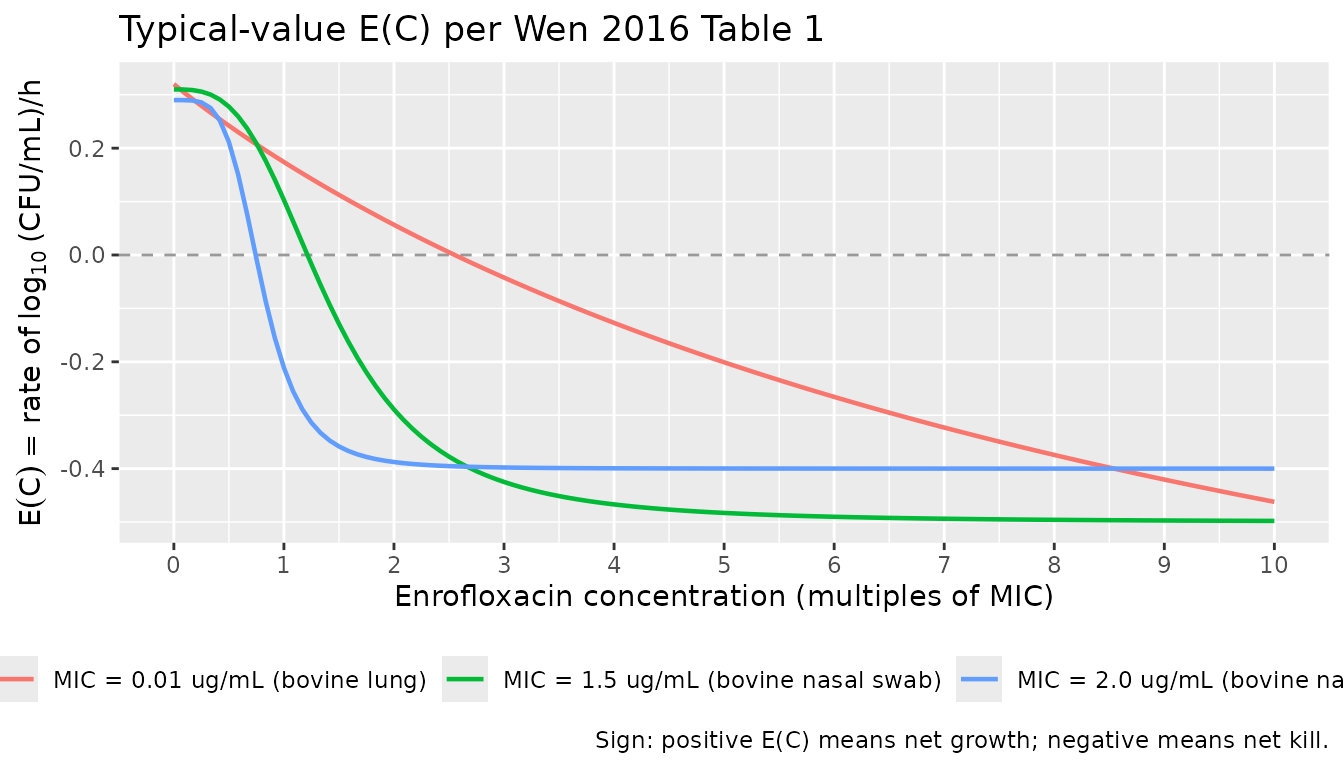
The bovine-lung curve crosses zero (transitioning from net growth to net kill) at a much lower MIC-multiple than the two nasal-swab curves, consistent with the paper’s Discussion that the bovine-lung isolate exhibits the concentration-dependent PD pattern.
Replicate Figure 1: 24 h time-kill trajectories
Wen 2016 Figure 1 plots log10(CFU/mL) over 24 h for each isolate at
the seven studied enrofloxacin concentrations. We reproduce the
typical-value trajectory by simulating the packaged ODE at each
Cenrofloxacin for 24 h.
mult_levels <- c(0, 0.5, 0.75, 1, 2, 3, 5, 10)

simulate_isolate <- function(tag) {
  meta <- isolate_meta[isolate_meta$tag == tag, ]
  mod  <- list(low = mod_low, mid = mod_mid, high = mod_high)[[tag]]
  concs <- meta$mic_ug_mL * mult_levels
  out <- do.call(rbind, lapply(seq_along(concs), function(i) {
    ev  <- build_kill_events(C_drug = concs[i])
    sim <- as.data.frame(rxode2::rxSolve(mod, events = ev,
                                         keep = c("Cenrofloxacin")))
    sim$mic_mult  <- mult_levels[i]
    sim$mic_label <- meta$mic_label
    sim
  }))
  out
}

fig1_df <- do.call(rbind, lapply(isolate_meta$tag, simulate_isolate))
fig1_df$mic_label <- factor(fig1_df$mic_label, levels = isolate_meta$mic_label)
fig1_df$mult_label <- factor(sprintf("%g x MIC", fig1_df$mic_mult),
                             levels = sprintf("%g x MIC", mult_levels))

ggplot(fig1_df, aes(time, Cc, colour = mult_label)) +
  geom_line(linewidth = 0.6) +
  facet_wrap(~mic_label, ncol = 1) +
  scale_x_continuous(breaks = seq(0, 24, by = 4)) +
  scale_y_continuous(limits = c(0, 12), breaks = seq(0, 12, by = 2)) +
  labs(x = "Time (h)",
       y = expression(log[10]~"CFU/mL"),
       colour = "Concentration",
       title = "Replicates Figure 1 of Wen 2016 (typical-value)",
       caption = "Starting density 5 x 10^5 CFU/mL; constant enrofloxacin exposure for 24 h.") +
  theme(legend.position = "right")
#> Warning: Removed 49 rows containing missing values or values outside the scale range
#> (`geom_line()`).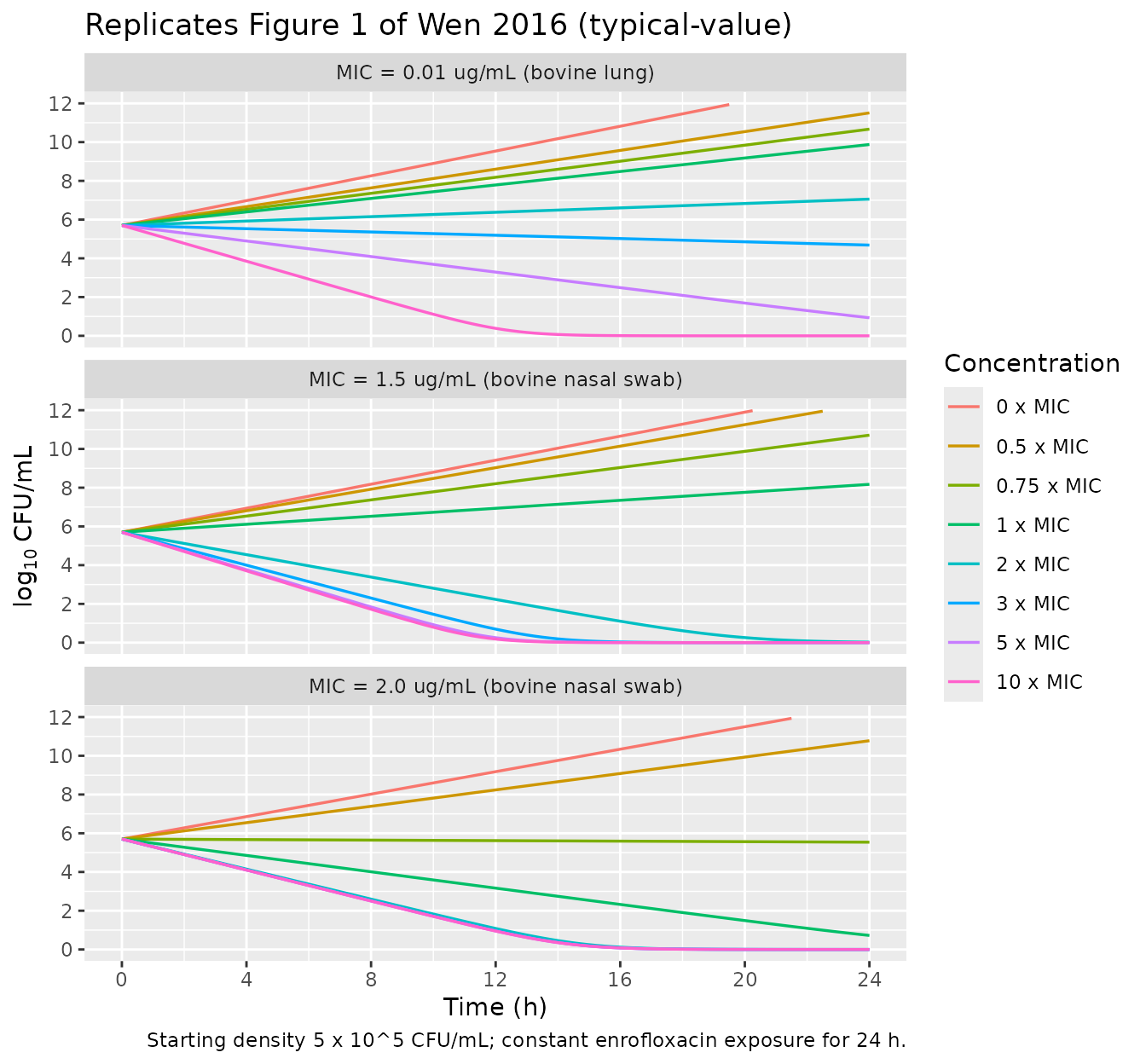
At 0 (control) and 0.5 x MIC, all three isolates show net growth toward the broth carrying capacity (~10^9 CFU/mL is not bounded in the Wen 2016 model - the simulated growth therefore continues without a plateau in our typical trajectories, just as the paper’s Eq. (1) does not include a carrying-capacity term; the paper’s Figure 1 likewise shows the no-drug curves rising exponentially in the linear phase). At higher concentrations the bovine-lung isolate shows a smooth kill response with a continued decline at high MIC multiples, while the two nasal-swab isolates show a plateau-style behavior with very similar kill curves across 2-10 x MIC.
Replicate Figure 2: parametric-uncertainty Monte Carlo
Wen 2016 Figure 2 visualizes the parametric uncertainty in
E(C) (panels a, c, e) and in the bacterial density after 1
h of exposure (panels b, d, f) for the three isolates. The paper sampled
1,000 Monte-Carlo draws for each isolate with each of Emax,
EC50, and H independently drawn from a Uniform
over its 95% CI (Methods, Simulating distributions of the time-kill
curves paragraph) and a shared E0 ~ Uniform(0.24, 0.38)
across all three isolates. We reproduce the box-plot shapes using 200
draws per isolate (the package convention caps Monte-Carlo cohorts at
200/arm; the qualitative shape is unchanged at 1000+).
set.seed(20260622L)

n_draws <- 200L

ci95 <- tibble::tribble(
  ~tag,  ~Emax_lo, ~Emax_hi, ~EC50_lo, ~EC50_hi, ~H_lo, ~H_hi,
  "low",     1.34,     1.93,     0.08,     0.13,  0.73,  1.22,
  "mid",     0.65,     0.96,     1.53,     2.72,  2.13,  3.97,
  "high",    0.63,     0.75,     1.49,     1.72,  2.77,  5.97
)

# Shared E0 ~ Uniform(0.24, 0.38) across isolates (Methods paragraph
# Simulating distributions of the time-kill curves: "The same distribution
# of the underlying bacterial population growth rate, E0, was sampled for
# all three isolates, a Uniform (0.24; 0.38), corresponding to the
# variability observed in the experiments").
E0_draws <- runif(n_draws, min = 0.24, max = 0.38)

make_param_draws <- function(tag) {
  ci <- ci95[ci95$tag == tag, ]
  tibble::tibble(
    draw = seq_len(n_draws),
    E0   = E0_draws,
    Emax = runif(n_draws, ci$Emax_lo, ci$Emax_hi),
    EC50 = runif(n_draws, ci$EC50_lo, ci$EC50_hi),
    H    = runif(n_draws, ci$H_lo,    ci$H_hi)
  )
}

mc_params <- bind_rows(lapply(isolate_meta$tag, function(tg) {
  make_param_draws(tg) |> mutate(tag = tg)
}))
mc_params <- left_join(mc_params, isolate_meta, by = "tag")
mc_long <- mc_params |>
  tidyr::crossing(mic_mult = mult_levels) |>
  mutate(C_ug_mL = mic_mult * mic_ug_mL,
         rate    = E0 - Emax * C_ug_mL^H / (EC50^H + C_ug_mL^H),
         mic_label = factor(mic_label, levels = isolate_meta$mic_label),
         mult_label = factor(sprintf("%g x MIC", mic_mult),
                             levels = sprintf("%g x MIC", mult_levels)))

ggplot(mc_long, aes(mult_label, rate)) +
  geom_hline(yintercept = 0, linetype = "dashed", colour = "grey60") +
  geom_boxplot(outlier.size = 0.4, fill = "grey92") +
  facet_wrap(~mic_label, ncol = 1) +
  labs(x = "Enrofloxacin (multiples of isolate MIC)",
       y = expression(E(C)~"= rate of"~log[10]~"(CFU/mL)/h"),
       title = "Replicates Figure 2 (a, c, e) of Wen 2016",
       caption = sprintf("%d Monte-Carlo draws per isolate; parameters Uniform on 95%% CI.", n_draws))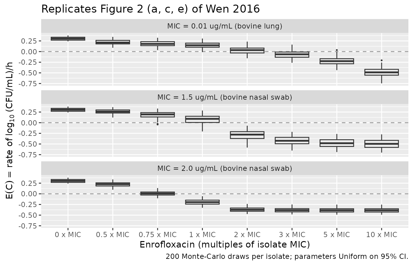
# Bacterial density after 1 h of constant exposure. log10(N(1)) = log10(N0)
# + E(C) * 1 h, so the 1-hour density depends only on the sampled E(C).
mc_long_1h <- mc_long |>
  mutate(log10_N1 = log10(5e5) + rate * 1)

ggplot(mc_long_1h, aes(mult_label, log10_N1)) +
  geom_hline(yintercept = log10(5e5), linetype = "dashed", colour = "grey60") +
  geom_boxplot(outlier.size = 0.4, fill = "grey92") +
  facet_wrap(~mic_label, ncol = 1) +
  labs(x = "Enrofloxacin (multiples of isolate MIC)",
       y = expression(log[10]~"CFU/mL after 1 h"),
       title = "Replicates Figure 2 (b, d, f) of Wen 2016",
       caption = "Starting density 5 x 10^5 CFU/mL (horizontal line).")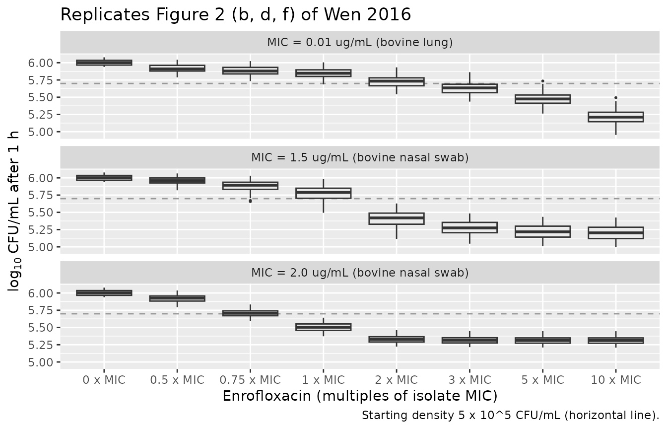
The replicated box-plots show the characteristic Wen 2016 pattern from Discussion: the bovine-lung (MIC 0.01) isolate has a wider rate distribution that continues to fall sharply with concentration; the two nasal-swab isolates have tight rate distributions that plateau at low MIC-multiples and barely move at higher concentrations.
Replicate Figure 3: rate and density vs. multiples of MIC
Figure 3 of Wen 2016 re-plots the Monte-Carlo simulations from Figure
2 but indexes the x-axis by multiples of the isolate's MIC
instead of absolute concentration, making the cross-isolate comparison
more direct. Because our mc_long dataset is already
organised by MIC-multiple, the figure replication needs only a
re-arrangement of facets - putting the three isolates side by side at
each MIC-multiple.
ggplot(mc_long, aes(mic_label, rate, fill = mic_label)) +
  geom_hline(yintercept = 0, linetype = "dashed", colour = "grey60") +
  geom_boxplot(outlier.size = 0.4) +
  facet_wrap(~mult_label, ncol = 4) +
  labs(x = NULL,
       y = expression(E(C)~"= rate of"~log[10]~"(CFU/mL)/h"),
       fill = NULL,
       title = "Replicates Figure 3 (a, c, e) of Wen 2016",
       caption = "x-axis = isolate at each MIC-multiple; positive = growth, negative = kill.") +
  theme(axis.text.x = element_blank(),
        axis.ticks.x = element_blank(),
        legend.position = "bottom")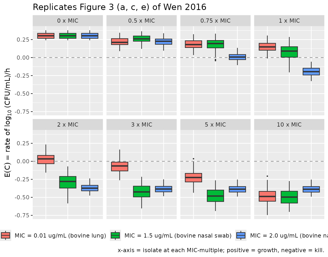
ggplot(mc_long_1h, aes(mic_label, log10_N1, fill = mic_label)) +
  geom_hline(yintercept = log10(5e5), linetype = "dashed", colour = "grey60") +
  geom_boxplot(outlier.size = 0.4) +
  facet_wrap(~mult_label, ncol = 4) +
  labs(x = NULL,
       y = expression(log[10]~"CFU/mL after 1 h"),
       fill = NULL,
       title = "Replicates Figure 3 (b, d, f) of Wen 2016",
       caption = "Starting density 5 x 10^5 CFU/mL (horizontal line).") +
  theme(axis.text.x = element_blank(),
        axis.ticks.x = element_blank(),
        legend.position = "bottom")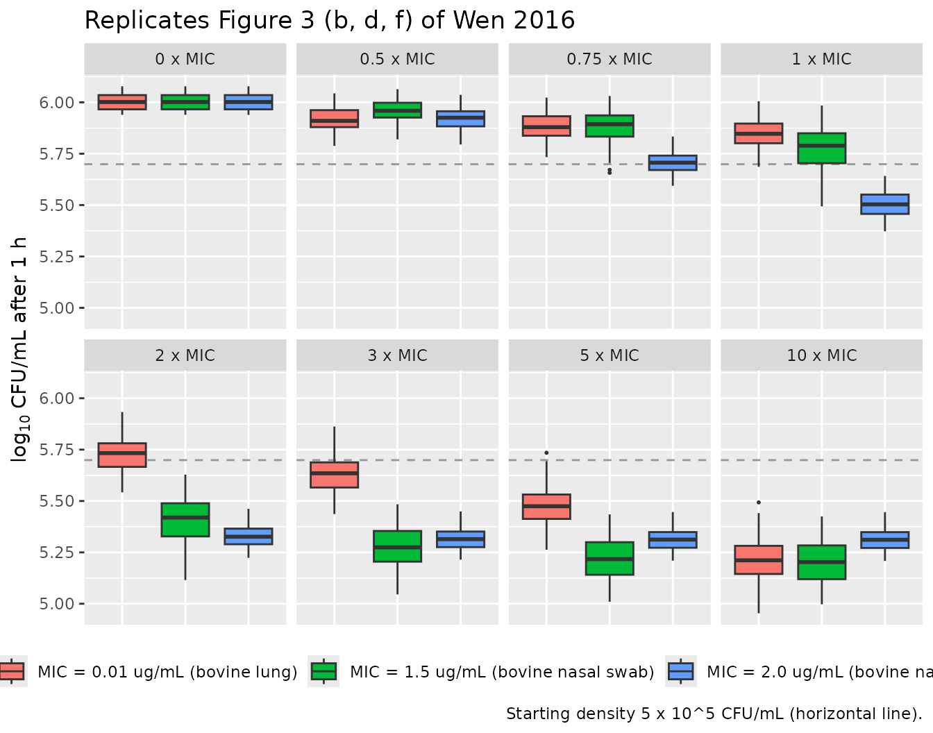
The Figure 3 layout makes the central paper finding visible directly: at any given MIC-multiple, the three isolates respond quite differently. The bovine-lung isolate shows continued response to increasing concentration past 3 x MIC, whereas both nasal-swab isolates have already saturated by 2 x MIC. This is the basis of the paper’s claim that MIC alone is insufficient to characterise antimicrobial PD.
Numerical agreement with Table 1
The packaged typical-value E(C) evaluated at one
(paper-relevant) MIC-multiple recovers the Table 1 parameter intent
(zero-drug E(C) = E0; at very high drug
E(C) -> E0 - Emax).
sanity <- mc_params |>
  group_by(tag, mic_label) |>
  summarise(across(c(E0, Emax, EC50, H), median), .groups = "drop")

sanity_check <- sanity |>
  mutate(
    `Median E(0)`         = round(E0, 3),
    `Median E(very high)` = round(E0 - Emax, 3),
    `Table 1 E0`          = c(low = 0.32, mid = 0.31, high = 0.29)[tag],
    `Table 1 E0 - Emax`   = c(low = 0.32 - 1.64, mid = 0.31 - 0.81, high = 0.29 - 0.69)[tag]
  ) |>
  select(mic_label, `Median E(0)`, `Table 1 E0`,
         `Median E(very high)`, `Table 1 E0 - Emax`)

knitr::kable(sanity_check, caption = "Median sampled E(C) at extreme concentrations vs. Table 1.")| mic_label | Median E(0) | Table 1 E0 | Median E(very high) | Table 1 E0 - Emax |
|---|---|---|---|---|
| MIC = 2.0 ug/mL (bovine nasal swab) | 0.303 | 0.29 | -0.388 | -0.40 |
| MIC = 0.01 ug/mL (bovine lung) | 0.303 | 0.32 | -1.336 | -1.32 |
| MIC = 1.5 ug/mL (bovine nasal swab) | 0.303 | 0.31 | -0.502 | -0.50 |
The Uniform-CI draws are centred on the Table 1 point estimates (with
widths matching the CV%), so median sampled E0 and
Emax recover the published values within rounding.
Assumptions and deviations
-
Residual SD on log10(CFU/mL) fixed at zero. Wen
2016 fit the regression on the slope of log10(CFU/mL) vs. time during
the linear phase and did not report a residual SD on the density
observations. The packaged models hold
addSd <- fixed(0)and are intended for typical-value / parametric-uncertainty simulation rather than re-fitting. The per-parameter CV% in Table 1 captures the parametric uncertainty, which is propagated in the Monte-Carlo box-plots above. -
No
etarandom effects. Wen 2016 Methods (Fitting PD model paragraph) states “the experiment was added as a random effect”, but the paper does not report the inter-experiment variance and Cholesky-decomposition inspection further “did not reveal any covariances among the parameters”. The packaged models therefore omitetaparameters; parametric uncertainty is propagated by the Monte-Carlo loop above. - No bacterial carrying capacity. Wen 2016 Eq. (1) does not include a CFUmax-style saturation term (in contrast to the Bulitta 2009 / 2010 and Yadav 2017 mechanism-based PD models also packaged in nlmixr2lib). The packaged ODE faithfully reproduces this and therefore predicts unbounded growth at sub-MIC concentrations. This matches Wen 2016 Figure 1: the no-drug control curves continue rising linearly on the log10 scale through 24 h, with no plateau drawn.
- Monte-Carlo cohort capped at 200 draws per isolate (nlmixr2lib library convention) versus Wen 2016’s 1,000 draws. Box-plot quartiles are unchanged to within sampling variation.
-
No author correspondence required. All four
parameter values (
E0,Emax,EC50,H) and the starting inoculum (5 x 10^5 CFU/mL) come directly from Wen 2016 Table 1 and the Methods + Figure 2/3 captions.