Glasdegib overall survival in AML (Lin 2020)
Source:vignettes/articles/Lin_2020_glasdegib_AML_overall_survival.Rmd
Lin_2020_glasdegib_AML_overall_survival.RmdModel and source
- Citation: Lin S, Shaik N, Chan G, Cortes JE, Ruiz-Garcia A. An evaluation of overall survival in patients with newly diagnosed acute myeloid leukemia and the relationship with glasdegib treatment and exposure. Cancer Chemother Pharmacol. 2020;86(4):451-459.
- Article: https://doi.org/10.1007/s00280-020-04132-x
- Trial: BRIGHT AML 1003, ClinicalTrials.gov NCT01546038
This vignette packages and validates three parametric exponential time-to-event (TTE) overall-survival (OS) models from Lin 2020 of the BRIGHT AML 1003 Phase 1b/2 trial in older adults with newly diagnosed AML who were ineligible for intensive chemotherapy:
-
Lin_2020_glasdegib_treatment– Phase 2 treatment-response analysis (n = 116; glasdegib + LDAC vs LDAC alone). Treatment arm is the only retained covariate. -
Lin_2020_glasdegib_exposure– Phase 2 exposure-response analysis (n = 75; glasdegib + LDAC subset with PK). Intercept-only exponential; no glasdegib exposure metric and no covariate was significant. -
Lin_2020_glasdegib_decitabine– exploratory pooled Phase 1b + Phase 2 analysis (n = 162) including the small glasdegib + decitabine cohort (n = 7) alongside glasdegib + LDAC (n = 117) and LDAC alone (n = 38).
All three were fit in NONMEM 7.3.0 with the likelihood-based
parametric TTE formulation (no estimated IIV, no residual error). For
each, the hazard is constant in time (exponential distribution) and
modulated multiplicatively by treatment arm where applicable. nlmixr2lib
expresses these via the canonical TTE pattern
d/dt(cumhaz) = hazard; sur = exp(-cumhaz).
Population
Phase 2 of BRIGHT AML 1003 randomised 116 older adults (>= 55 years) with newly diagnosed AML who were ineligible for intensive chemotherapy: 78 to glasdegib 100 mg orally once daily plus low-dose cytarabine (LDAC; 20 mg SC BID for 10 days per 28-day cycle), and 38 to LDAC alone. Lin 2020 Table 1 reports a median age of 76 years (range 58-92), median weight 78.2 kg (47.5-118.0), 71% male, 97% White (with 1% Black and 2% Asian); median baseline creatinine clearance (Cockcroft-Gault) of 62.7 mL/min, suggesting mild renal impairment in most patients; 52% had secondary AML and 40% had poor cytogenetic risk. Phase 1b added 39 patients to Arm A (glasdegib + LDAC) and 7 patients to Arm B (glasdegib + decitabine; 5 AML + 2 MDS), giving the n = 162 exploratory pooled cohort.
Source trace
The full per-parameter origin is recorded as in-file comments next to
each ini() entry in
inst/modeldb/therapeuticArea/oncology/Lin_2020_glasdegib_*.R.
The tables below collect them.
Lin_2020_glasdegib_treatment (Phase 2 treatment-response, n = 116)
| Equation / parameter | Value | Source location |
|---|---|---|
S(t) = exp(-lambda * (1 + theta_ldac_alone * LDAC_alone) * t) |
n/a | Lin 2020 Results page 4 typeset equation; Fig. 1b annotation |
llam_haz (lambda for glasdegib + LDAC) |
log(0.00253) (1/day) | Lin 2020 page 4: 0.00253, RSE 13.82% |
e_ldac_alone (theta_ldac_alone) |
1.376 | Lin 2020 page 4: 1.376, RSE 37.74% (138% increase in base hazard for LDAC alone) |
| Hazard ratio glasdegib + LDAC vs LDAC alone | 0.421 (computed) | Lin 2020 abstract / page 4: published HR 0.42 (95% CI 0.28-0.66) |
| Estimated IIV on lambda | none | Source NONMEM TTE fit with no subject-level random effects |
| Residual error | none | Source uses NONMEM LIKE / F_FLAG
parametric-TTE branch |
Lin_2020_glasdegib_exposure (Phase 2 exposure-response subset, n = 75)
| Equation / parameter | Value | Source location |
|---|---|---|
S(t) = exp(-lambda * t) |
n/a | Lin 2020 Results page 5; Fig. 3 annotation |
llam_haz (lambda) |
log(0.00246) (1/day) | Lin 2020 page 5: 0.00246, RSE 14.19% |
| Covariates retained after SCM backward elimination | none | Lin 2020 page 5: seven glasdegib exposure metrics (raw and log-transformed) plus ECOG and cytogenetic risk were tested; none survived |
Lin_2020_glasdegib_decitabine (exploratory pooled Phase 1b + Phase 2, n = 162)
| Equation / parameter | Value | Source location |
|---|---|---|
S(t) = exp(-lambda * (1 - theta_gl_ldac * GL_LDAC_arm) * (1 - theta_gl_dec * GL_DEC_arm) * t) |
n/a | Lin 2020 Results page 6 typeset equation |
llam_haz (lambda for LDAC alone) |
log(0.00540) (1/day) | Lin 2020 page 6: 0.00540, RSE 14.1% |
e_gl_ldac_haz (theta_gl_ldac) |
0.480 | Lin 2020 page 6 equation: 0.480 (= 48.0% hazard reduction for glasdegib + LDAC) |
e_gl_dec_haz (theta_gl_dec) |
0.618 | Lin 2020 page 6 prose / equation: ~61.8% hazard reduction for glasdegib + decitabine (95% CI of change in base hazard -95.0% to -28.6%) |
Virtual cohort
The published trial-level individual data are not redistributed. The
virtual cohort below assigns each subject to one of the three trial arms
in proportions matching the BRIGHT AML 1003 pooled cohort, and observes
the survival probability sur on a daily grid out to 40
months (1216 days). The exponential-hazard structure produces a
deterministic typical-value S(t) per arm; per the Lin 2020
source NONMEM fit, no subject-level IIV is added, so all subjects in an
arm follow the same S(t) trajectory.
Per the vignette template’s cohort-size cap, each arm uses <= 200 subjects.
set.seed(20260624)

# One observation row per subject per visit day. Observation grid: every 14
# days out to 1216 days (~40 months), matching the Lin 2020 Fig. 1 / Fig. 4
# x-axis range; a time = 0 anchor row is included.
obs_times <- c(0, seq(14, 1216, by = 14))

make_arm <- function(arm_label, n, id_offset, CONMED_GLASDEGIB, CONMED_DECITABINE) {
  ids <- id_offset + seq_len(n)
  tidyr::crossing(
    id = ids,
    time = obs_times
  ) |>
    dplyr::mutate(
      evid  = 0L,
      amt   = 0,
      cmt   = NA_character_,
      arm   = arm_label,
      CONMED_GLASDEGIB  = CONMED_GLASDEGIB,
      CONMED_DECITABINE = CONMED_DECITABINE
    ) |>
    dplyr::select(id, time, evid, amt, cmt, arm,
                  CONMED_GLASDEGIB, CONMED_DECITABINE)
}

events <- dplyr::bind_rows(
  make_arm("LDAC alone",            n = 38,  id_offset =   0L,
           CONMED_GLASDEGIB = 0, CONMED_DECITABINE = 0),
  make_arm("Glasdegib + LDAC",      n = 117, id_offset = 100L,
           CONMED_GLASDEGIB = 1, CONMED_DECITABINE = 0),
  make_arm("Glasdegib + decitabine", n = 7,   id_offset = 300L,
           CONMED_GLASDEGIB = 1, CONMED_DECITABINE = 1)
)

stopifnot(!anyDuplicated(unique(events[, c("id", "time", "evid")])))
cat("Arms:\n"); print(events |> dplyr::distinct(id, arm) |> dplyr::count(arm))
#> Arms:
#> # A tibble: 3 × 2
#>   arm                        n
#>   <chr>                  <int>
#> 1 Glasdegib + LDAC         117
#> 2 Glasdegib + decitabine     7
#> 3 LDAC alone                38
Treatment-response model (Lin_2020_glasdegib_treatment, n = 116)
The treatment-response model uses only CONMED_GLASDEGIB
(1 = glasdegib + LDAC arm, 0 = LDAC alone). Subjects in the glasdegib +
decitabine arm of the exploratory cohort are not part of this analysis,
so the simulation below is restricted to the LDAC alone and glasdegib +
LDAC arms.
mod_trt <- readModelDb("Lin_2020_glasdegib_treatment")

events_trt <- events |> dplyr::filter(arm != "Glasdegib + decitabine")

sim_trt <- rxode2::rxSolve(mod_trt, events = events_trt, keep = c("arm")) |>
  as.data.frame()

# All subjects within an arm share the same typical-value S(t); pick one.
typ_trt <- sim_trt |>
  dplyr::group_by(arm, time) |>
  dplyr::summarise(sur = mean(sur), hazard = mean(hazard), .groups = "drop")
# Replicates Fig. 1b of Lin 2020: predicted S(t) for the final treatment-
# response model by treatment arm.
month_per_day <- 12 / 365.25

ggplot(typ_trt, aes(time * month_per_day, sur, colour = arm)) +
  geom_line(linewidth = 1) +
  scale_x_continuous(breaks = seq(0, 40, by = 10), limits = c(0, 40)) +
  scale_y_continuous(limits = c(0, 1), labels = scales::percent_format(accuracy = 1)) +
  labs(x = "Time (months)", y = "Probability of OS",
       title = "Replicates Fig. 1b of Lin 2020 -- final treatment-response model",
       caption = "Glasdegib + LDAC: S(t) = exp(-0.00253 t). LDAC alone: S(t) = exp(-0.00601 t).",
       colour = "Treatment arm")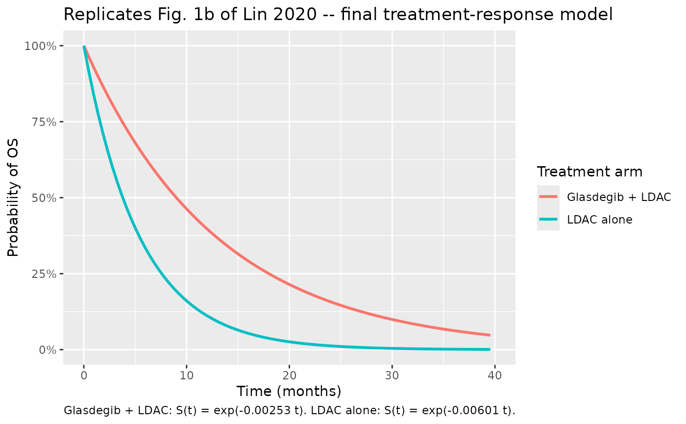
Validation against the published survival functions and median OS
Both arms have an exponential survival function
S(t) = exp(-h * t) with analytical median OS
ln(2) / h. The table below compares the implementation
against the published hazards and median OS.
trt_check <- tibble::tribble(
  ~arm,                ~h_published_per_day, ~h_simulated_per_day,
  "Glasdegib + LDAC",  0.00253,              typ_trt |> dplyr::filter(arm == "Glasdegib + LDAC", time == 0) |> dplyr::pull(hazard),
  "LDAC alone",        0.00253 * (1 + 1.376),
                                              typ_trt |> dplyr::filter(arm == "LDAC alone", time == 0) |> dplyr::pull(hazard)
) |>
  dplyr::mutate(
    median_OS_pub_months = log(2) / h_published_per_day * month_per_day,
    median_OS_sim_months = log(2) / h_simulated_per_day * month_per_day,
    abs_pct_diff_h       = abs(h_simulated_per_day - h_published_per_day) /
                           h_published_per_day * 100
  )
knitr::kable(trt_check, digits = 5,
caption = "Treatment-response model: published vs simulated hazards and median OS.")| arm | h_published_per_day | h_simulated_per_day | median_OS_pub_months | median_OS_sim_months | abs_pct_diff_h |
|---|---|---|---|---|---|
| Glasdegib + LDAC | 0.00253 | 0.00253 | 9.00111 | 9.00111 | 0 |
| LDAC alone | 0.00601 | 0.00601 | 3.78835 | 3.78835 | 0 |
# Hard checks: simulated hazards within 0.1% of published, and median OS
# difference within 5 months of the paper's headline (~5 month gain).
stopifnot(all(trt_check$abs_pct_diff_h < 0.1))
stopifnot(abs(trt_check$median_OS_pub_months[1] - trt_check$median_OS_pub_months[2]) > 4)
stopifnot(abs(trt_check$median_OS_pub_months[1] - trt_check$median_OS_pub_months[2]) < 6)

# Hazard ratio glasdegib + LDAC vs LDAC alone should match the published 0.42.
hr_sim <- trt_check$h_simulated_per_day[1] / trt_check$h_simulated_per_day[2]
cat(sprintf("Hazard ratio glasdegib+LDAC vs LDAC alone: %.3f (paper: 0.42 [0.28-0.66])\n",
            hr_sim))
#> Hazard ratio glasdegib+LDAC vs LDAC alone: 0.421 (paper: 0.42 [0.28-0.66])
stopifnot(abs(hr_sim - 0.42) < 0.01)
Exposure-response model (Lin_2020_glasdegib_exposure, n = 75)
This is an intercept-only exponential model fit to the n = 75 glasdegib + LDAC subset with PK data. The hazard does not depend on any covariate.
mod_exp <- readModelDb("Lin_2020_glasdegib_exposure")

# A single typical subject is sufficient because no covariate enters the
# hazard.
events_exp <- tibble::tibble(
  id   = 1L,
  time = obs_times,
  evid = 0L,
  amt  = 0,
  cmt  = NA_character_
)
sim_exp <- rxode2::rxSolve(mod_exp, events = events_exp) |> as.data.frame()
# Replicates Fig. 3 of Lin 2020: predicted S(t) for the final exposure-
# response model (intercept-only).
ggplot(sim_exp, aes(time * month_per_day, sur)) +
  geom_line(linewidth = 1, colour = "firebrick") +
  scale_x_continuous(breaks = seq(0, 40, by = 10), limits = c(0, 40)) +
  scale_y_continuous(limits = c(0, 1), labels = scales::percent_format(accuracy = 1)) +
  labs(x = "Time (months)", y = "Probability of OS",
       title = "Replicates Fig. 3 of Lin 2020 -- final exposure-response model",
       caption = "S(t) = exp(-0.00246 t).")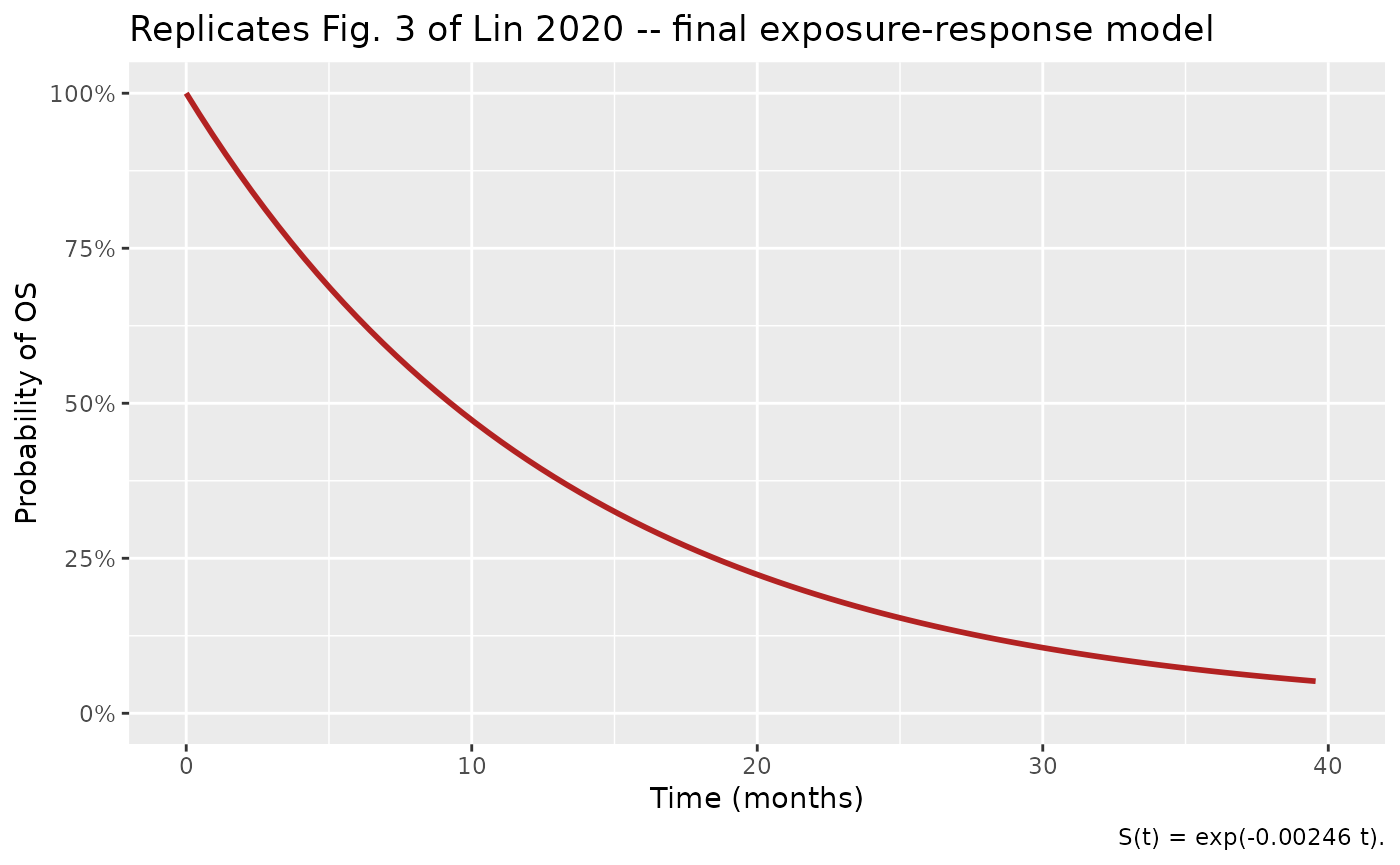
h_exp_pub <- 0.00246
h_exp_sim <- sim_exp$hazard[1]
exp_check <- tibble::tibble(
  source              = c("published", "simulated"),
  h_per_day           = c(h_exp_pub, h_exp_sim),
  median_OS_months    = log(2) / c(h_exp_pub, h_exp_sim) * month_per_day
)
knitr::kable(exp_check, digits = 5,
caption = "Exposure-response model: published vs simulated hazard and median OS.")| source | h_per_day | median_OS_months |
|---|---|---|
| published | 0.00246 | 9.25724 |
| simulated | 0.00246 | 9.25724 |
Exploratory pooled model (Lin_2020_glasdegib_decitabine, n = 162)
The exploratory model includes all three trial arms. The published
per-arm median OS is approximately 11.1 months for glasdegib +
decitabine, 9.1 months for glasdegib + LDAC (computed from
log(2) / (0.00540 * (1 - 0.480))), and 4.2 months for LDAC
alone (computed from log(2) / 0.00540).
mod_dec <- readModelDb("Lin_2020_glasdegib_decitabine")

sim_dec <- rxode2::rxSolve(mod_dec, events = events, keep = c("arm")) |>
  as.data.frame()

typ_dec <- sim_dec |>
  dplyr::group_by(arm, time) |>
  dplyr::summarise(sur = mean(sur), hazard = mean(hazard), .groups = "drop")
# Replicates Fig. 4 of Lin 2020: predicted S(t) for the exploratory three-arm
# model.
arm_levels <- c("LDAC alone", "Glasdegib + LDAC", "Glasdegib + decitabine")
ggplot(typ_dec |> dplyr::mutate(arm = factor(arm, levels = arm_levels)),
       aes(time * month_per_day, sur, colour = arm)) +
  geom_line(linewidth = 1) +
  scale_x_continuous(breaks = seq(0, 40, by = 10), limits = c(0, 40)) +
  scale_y_continuous(limits = c(0, 1), labels = scales::percent_format(accuracy = 1)) +
  labs(x = "Time (months)", y = "Probability of OS",
       title = "Replicates Fig. 4 of Lin 2020 -- exploratory three-arm model",
       caption = paste("LDAC alone: S(t) = exp(-0.00540 t).",
                       "Glasdegib + LDAC: S(t) = exp(-0.00540*0.520 t).",
                       "Glasdegib + decitabine: S(t) = exp(-0.00540*0.382 t)."),
       colour = "Treatment arm")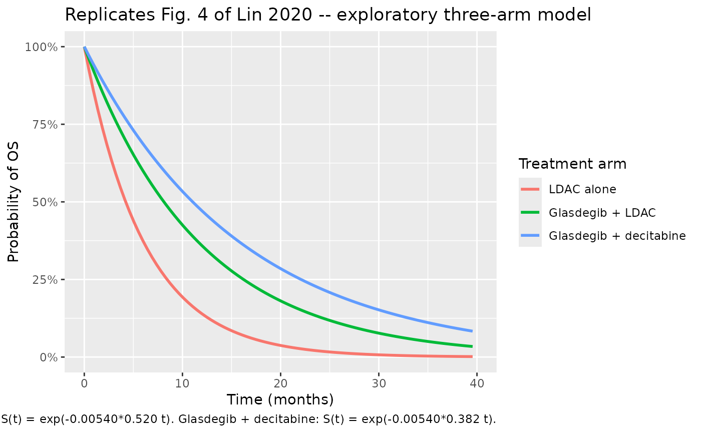
h_ldac     <- 0.00540
h_gl_ldac  <- 0.00540 * (1 - 0.480)
h_gl_dec   <- 0.00540 * (1 - 0.618)

dec_check <- tibble::tribble(
  ~arm,                     ~h_published_per_day, ~h_simulated_per_day,
  "LDAC alone",             h_ldac,
                            typ_dec |> dplyr::filter(arm == "LDAC alone", time == 0) |> dplyr::pull(hazard),
  "Glasdegib + LDAC",       h_gl_ldac,
                            typ_dec |> dplyr::filter(arm == "Glasdegib + LDAC", time == 0) |> dplyr::pull(hazard),
  "Glasdegib + decitabine", h_gl_dec,
                            typ_dec |> dplyr::filter(arm == "Glasdegib + decitabine", time == 0) |> dplyr::pull(hazard)
) |>
  dplyr::mutate(
    median_OS_pub_months = log(2) / h_published_per_day * month_per_day,
    median_OS_sim_months = log(2) / h_simulated_per_day * month_per_day,
    abs_pct_diff_h       = abs(h_simulated_per_day - h_published_per_day) /
                           h_published_per_day * 100
  )

knitr::kable(dec_check, digits = 5,
caption = "Exploratory three-arm model: published vs simulated hazards and median OS.")| arm | h_published_per_day | h_simulated_per_day | median_OS_pub_months | median_OS_sim_months | abs_pct_diff_h |
|---|---|---|---|---|---|
| LDAC alone | 0.00540 | 0.00540 | 4.21719 | 4.21719 | 0 |
| Glasdegib + LDAC | 0.00281 | 0.00281 | 8.10997 | 8.10997 | 0 |
| Glasdegib + decitabine | 0.00206 | 0.00206 | 11.03975 | 11.03975 | 0 |
stopifnot(all(dec_check$abs_pct_diff_h < 0.1))

# Paper reports glasdegib + decitabine median OS = 11.1 months. Computed
# value should agree within 0.5 months.
dec_median <- dec_check$median_OS_pub_months[dec_check$arm == "Glasdegib + decitabine"]
cat(sprintf("Glasdegib + decitabine median OS: %.2f months (paper: 11.1 months)\n",
            dec_median))
#> Glasdegib + decitabine median OS: 11.04 months (paper: 11.1 months)
stopifnot(abs(dec_median - 11.1) < 0.5)
Assumptions and deviations
Treatment arm encoded via canonical drug indicators. Lin 2020 expresses the treatment-response model with the binary covariate
LDAC_alone(1 = LDAC alone, 0 = glasdegib + LDAC), and the exploratory three-arm model with two binary covariatesglasdegib+LDACandglasdegib+decitabine(reference = LDAC alone). The nlmixr2lib model files use the canonical covariatesCONMED_GLASDEGIBandCONMED_DECITABINE(1 if the named drug is present in the subject’s treatment regimen) and derive the paper’s arm indicators insidemodel()–ldac_alone = 1 - CONMED_GLASDEGIBfor the treatment-response model, andgl_ldac_arm = CONMED_GLASDEGIB * (1 - CONMED_DECITABINE),gl_dec_arm = CONMED_GLASDEGIB * CONMED_DECITABINEfor the exploratory model. Published parameter values (lambda, theta_ldac_alone, theta_gl_ldac, theta_gl_dec) are preserved verbatim; the substitution is purely a column-naming choice that aligns with the canonical register.No estimated IIV. All three source NONMEM runs were fit without subject-level random effects (parametric population TTE). The packaged models therefore produce a single typical-value
S(t)per covariate setting; per-subject survival trajectories within an arm are identical.No residual error. The source NONMEM
$ERROR/$ESTframework for parametric TTE uses theLIKE/F_FLAGbranch (the likelihood is the survival / event-density itself). The packaged models exposesurandhazardas derived outputs intended for forward simulation; downstream users who want stochastic event-time sampling should layer a survival- sampling step on top (e.g. inverse-CDF sampling of an exponential with ratehazard).Documented-but-unused covariates. All baseline demographics, baseline safety laboratory values, and disease characteristics that Lin 2020 screened in SCM forward inclusion but did not retain after backward elimination are documented in each model file’s
covariatesDataExcludedlist (with the cohort-level summary statistics from Table 1). ThecovariatesDataExcludedmechanism preserves the screening provenance without flagging the entries as model-required.Exposure-response cohort size. The exposure-response analysis (n = 75) is a strict subset of the treatment-response analysis glasdegib + LDAC arm (n = 78); the difference of 3 patients is those without available glasdegib PK information.
Phase 1b Arm A subjects. Phase 1b Arm A evaluated glasdegib at 100 or 200 mg QD plus LDAC; Phase 2 used the 100 mg QD dose. The exploratory pooled analysis pools both phases into the glasdegib + LDAC arm because the exposure-response analysis showed no significant glasdegib dose / exposure effect on OS. The packaged exploratory model encodes a single
CONMED_GLASDEGIB = 1for all glasdegib-containing subjects regardless of dose level.No errata. A search of the journal landing page, publisher corrections feed, and PubMed at extraction time (2026-06-24) found no errata or corrigenda for Lin 2020.