TMDD archetypes: full, QSS, and Michaelis-Menten approximations • nlmixr2lib

Overview

nlmixr2lib ships five canonical target-mediated drug disposition (TMDD) archetypes. They are intended as starting scaffolds for mAb PK modelling, not drug-specific fits; the initial estimates are plausible mAb-scale defaults.

Model	Structural form	Drug compartments	Target states
`PK_1cmt_tmdd_full`	Mager & Jusko 2001	depot + central	free `target` + `complex`
`PK_1cmt_tmdd_qss`	Gibiansky et al. 2008	depot + central	`total_target` (QSS algebraic)
`PK_1cmt_tmdd_mm`	Gibiansky et al. 2008	depot + central	none (saturable elimination)
`PK_2cmt_tmdd_qss`	Gibiansky et al. 2008	depot + central + peripheral1	`total_target` (QSS algebraic)
`PK_2cmt_tmdd_mm`	Gibiansky et al. 2008	depot + central + peripheral1	none (saturable elimination)

Source citations, stored in each model’s reference field:

vapply(
  c("PK_1cmt_tmdd_full", "PK_1cmt_tmdd_qss", "PK_1cmt_tmdd_mm",
    "PK_2cmt_tmdd_qss", "PK_2cmt_tmdd_mm"),
  function(nm) nlmixr2est::nlmixr(readModelDb(nm))$reference,
  character(1)
)
#>                                                                                                                                                                                                                PK_1cmt_tmdd_full 
#>                                          "Mager DE, Jusko WJ. General pharmacokinetic model for drugs exhibiting target-mediated drug disposition. J Pharmacokinet Pharmacodyn. 2001;28(6):507-532. doi:10.1023/A:1014414520282" 
#>                                                                                                                                                                                                                 PK_1cmt_tmdd_qss 
#> "Gibiansky L, Gibiansky E, Kakkar T, Ma P. Approximations of the target-mediated drug disposition model and identifiability of model parameters. J Pharmacokinet Pharmacodyn. 2008;35(5):573-591. doi:10.1007/s10928-008-9102-8" 
#>                                                                                                                                                                                                                  PK_1cmt_tmdd_mm 
#> "Gibiansky L, Gibiansky E, Kakkar T, Ma P. Approximations of the target-mediated drug disposition model and identifiability of model parameters. J Pharmacokinet Pharmacodyn. 2008;35(5):573-591. doi:10.1007/s10928-008-9102-8" 
#>                                                                                                                                                                                                                 PK_2cmt_tmdd_qss 
#> "Gibiansky L, Gibiansky E, Kakkar T, Ma P. Approximations of the target-mediated drug disposition model and identifiability of model parameters. J Pharmacokinet Pharmacodyn. 2008;35(5):573-591. doi:10.1007/s10928-008-9102-8" 
#>                                                                                                                                                                                                                  PK_2cmt_tmdd_mm 
#> "Gibiansky L, Gibiansky E, Kakkar T, Ma P. Approximations of the target-mediated drug disposition model and identifiability of model parameters. J Pharmacokinet Pharmacodyn. 2008;35(5):573-591. doi:10.1007/s10928-008-9102-8"

Articles:
- Mager & Jusko 2001 — https://doi.org/10.1023/A:1014414520282
- Gibiansky et al. 2008 — https://doi.org/10.1007/s10928-008-9102-8

Population and units

These are generic archetypes; no specific population is represented. Units are time = day, dosing = mg, concentration = mg/L. Free drug, free target, and drug-target complex are all carried as concentrations in mg/L so the rate constants are unit-consistent without a molecular-weight conversion. A user who prefers molar units (nM) can re-interpret the concentration-bearing parameters (lT0, lkon, lKss, lVm, propSd) in that system.

Initial estimates are plausible mAb-scale defaults (Mager & Jusko 2001 canonical TMDD behaviour; Davda 2014 linear-PK meta-analysis anchors for clearance/volume). They are not fit to any specific dataset; the per-field population$notes metadata in each model file states this explicitly.

Source trace

Per-parameter origin is recorded as an in-file comment next to each ini() entry in the model source under inst/modeldb/pharmacokinetics/PK_*_tmdd_*.R. The table below collects the equation references.

Parameter (symbol)	Mager & Jusko 2001	Gibiansky et al. 2008
CL, Vc (linear disposition)	Eq 1 (k_el * V, V)	Eq 8 / Eq 10 (k_el * V, V)
Vp, Q (peripheral, 2-cmt)	n/a	two-compartment extension (implicit)
Ka, F (absorption)	Eq 1 (input term)	Eq 6 (input term)
T0 = ksyn / kdeg	Eq 2 (R0)	Eq 9 (Rtot(0))
kdeg	Eq 2 (k_deg)	Eq 9 (k_deg)
kint	Eq 3 (k_int)	Eq 9 / Eq 10 (k_int)
kon, koff (full only)	Eq 1 (k_on, k_off)	n/a (eliminated by QSS / MM)
Kss = (koff + kint)/kon	n/a (full keeps kon/koff explicit)	Eq 7 (Kss)
Vm, Km (MM only)	n/a	Eq 10 (V_m = k_int * R0, K_m approx Kss)

Typical-value simulations

The three 1-compartment variants share the same drug-disposition parameters and differ only in how target binding is handled. The two 2-compartment variants add a peripheral distribution compartment for drug. The code below simulates each model with between-subject variability zeroed out (typical individual) over 56 days after a single SC dose and after repeated SC dosing.

solve_typical <- function(model_name, events) {
  ui <- nlmixr2est::nlmixr(readModelDb(model_name))
  ui_typ <- rxode2::zeroRe(ui)
  sim <- rxode2::rxSolve(ui_typ, events, returnType = "data.frame")
  sim$model <- model_name
  sim
}

Single-dose profiles (100 mg SC)

ev_single <- rxode2::et(amt = 100, cmt = "depot") |>
  rxode2::et(seq(0, 56, by = 0.25))

sims_single <- dplyr::bind_rows(lapply(
  c("PK_1cmt_tmdd_full", "PK_1cmt_tmdd_qss", "PK_1cmt_tmdd_mm",
    "PK_2cmt_tmdd_qss", "PK_2cmt_tmdd_mm"),
  solve_typical, events = ev_single
))
#> ℹ omega/sigma items treated as zero: 'etalcl', 'etalvc', 'etalka'
#> ℹ omega/sigma items treated as zero: 'etalcl', 'etalvc', 'etalka'
#> ℹ omega/sigma items treated as zero: 'etalcl', 'etalvc', 'etalka'
#> ℹ omega/sigma items treated as zero: 'etalcl', 'etalvc', 'etalka'
#> ℹ omega/sigma items treated as zero: 'etalcl', 'etalvc', 'etalka'

sims_single |>
  dplyr::mutate(structure = ifelse(grepl("1cmt", model), "1-compartment", "2-compartment"),
                variant   = sub("PK_._cmt_tmdd_", "", model)) |>
  ggplot(aes(time, Cc, colour = variant, linetype = structure)) +
  geom_line(linewidth = 0.6) +
  scale_y_log10() +
  labs(x = "Time (day)", y = expression(C[c] ~ "(mg/L)"),
       title = "Cc — 100 mg SC, typical-value simulation",
       caption = "The 1-cmt full and 1-cmt QSS curves overlay in the fast-binding, large-Kss regime.",
       colour = "variant", linetype = "structure")
#> Warning in scale_y_log10(): log-10 transformation introduced
#> infinite values.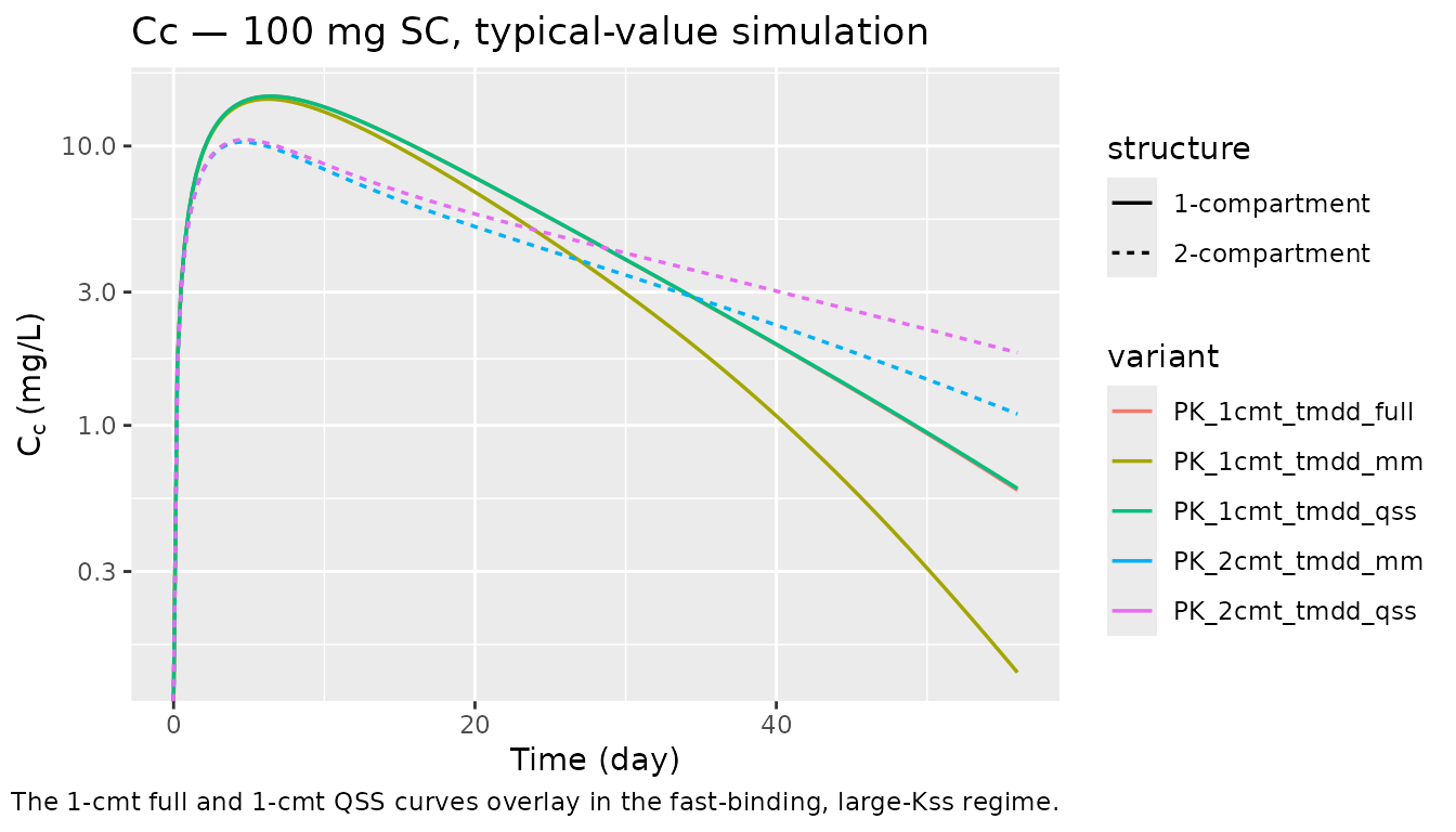

Target and complex trajectories (1-cmt models)

The full model carries target (free) and complex as explicit ODE states. The QSS model carries total_target = free + complex as a single state and derives the split algebraically. The MM model collapses target into a saturable elimination pathway and does not expose target state variables.

sim_full <- solve_typical("PK_1cmt_tmdd_full", ev_single)
#> ℹ omega/sigma items treated as zero: 'etalcl', 'etalvc', 'etalka'
sim_qss  <- solve_typical("PK_1cmt_tmdd_qss",  ev_single)
#> ℹ omega/sigma items treated as zero: 'etalcl', 'etalvc', 'etalka'

target_long <- dplyr::bind_rows(
  tibble::tibble(time = sim_full$time, value = sim_full$target,
                 species = "free target",          model = "full"),
  tibble::tibble(time = sim_full$time, value = sim_full$complex,
                 species = "drug-target complex",  model = "full"),
  tibble::tibble(time = sim_qss$time,
                 value = sim_qss$total_target - sim_qss$complex,
                 species = "free target",          model = "QSS"),
  tibble::tibble(time = sim_qss$time, value = sim_qss$complex,
                 species = "drug-target complex",  model = "QSS")
)

ggplot(target_long, aes(time, value, colour = model)) +
  geom_line(linewidth = 0.6) +
  facet_wrap(~ species, scales = "free_y") +
  labs(x = "Time (day)", y = "Concentration (mg/L)",
       title = "Target and complex — full vs QSS (1-cmt)")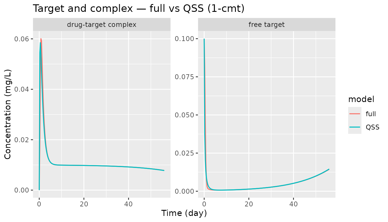

Repeated SC dosing — drug-concentration difference across structures

ev_multi <- rxode2::et(amt = 100, cmt = "depot", ii = 14, addl = 5) |>
  rxode2::et(seq(0, 100, by = 0.5))

sims_multi <- dplyr::bind_rows(lapply(
  c("PK_1cmt_tmdd_qss", "PK_2cmt_tmdd_qss",
    "PK_1cmt_tmdd_mm",  "PK_2cmt_tmdd_mm"),
  solve_typical, events = ev_multi
))
#> ℹ omega/sigma items treated as zero: 'etalcl', 'etalvc', 'etalka'
#> ℹ omega/sigma items treated as zero: 'etalcl', 'etalvc', 'etalka'
#> ℹ omega/sigma items treated as zero: 'etalcl', 'etalvc', 'etalka'
#> ℹ omega/sigma items treated as zero: 'etalcl', 'etalvc', 'etalka'

sims_multi |>
  ggplot(aes(time, Cc, colour = model)) +
  geom_line(linewidth = 0.6) +
  scale_y_log10() +
  labs(x = "Time (day)", y = expression(C[c] ~ "(mg/L)"),
       title = "Cc — 100 mg SC Q14D x 6, typical value")
#> Warning in scale_y_log10(): log-10 transformation introduced
#> infinite values.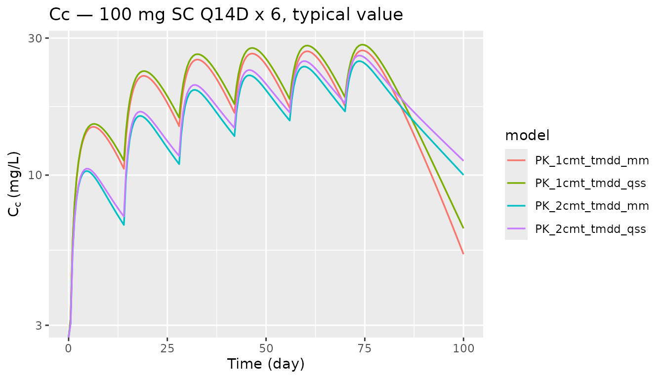

Regime-convergence check

The Gibiansky 2008 derivation shows that the QSS approximation should recover the full Mager–Jusko model when drug-target binding and unbinding are fast relative to internalization and drug disposition. Equivalently Kss = (koff + kint)/kon should be small relative to drug concentration for the approximation to hold.

The default parameter values put the model in that regime (kon = 1 L/mg/day, koff = 0.1 /day, kint = 1 /day so Kss = 1.1 mg/L, well below the Cc peak of ~15 mg/L for a 100-mg SC dose). The overlay of the full and QSS curves above is the asymptotic result.

Assumptions and deviations

Initial estimates are generic mAb-scale defaults, not derived from any specific trial. The archetypes are scaffolds; users must override the numeric starting values in ini() when fitting a real dataset.
All concentration-bearing quantities (drug, free target, complex) are in mg/L. The kon parameter has units L/(mg*day). For a given molecular weight, a conversion to the more conventional molar units (nM, 1/(nM*day)) is a multiplicative factor on T0, kon, and Kss.
The full model’s Cc is free drug concentration (Mager & Jusko 2001 convention). The QSS and MM models’ Cc is total drug concentration (Gibiansky 2008 convention) because the central compartment state holds the total drug amount in those reductions. Users whose assay reads total drug on the full model can compute it as Cc_total <- Cc + complex.
No population (IIV, residual error) simulation is shown here; the between-subject variance defaults in the models are placeholders. VPCs belong in drug-specific vignettes.
PKNCA validation is intentionally omitted: these archetypes do not target any published NCA table. Drug-specific TMDD vignettes (future specificDrugs/ entries) should include a full PKNCA comparison against their source tables.