Gastric emptying / CCK / GBE (Guiastrennec 2016)
Source:vignettes/articles/Guiastrennec_2016_gastric_emptying.Rmd
Guiastrennec_2016_gastric_emptying.RmdModel and source
- Citation: Guiastrennec B, Sonne DP, Hansen M, Bagger JI, Lund A, Rehfeld JF, Alskar O, Karlsson MO, Vilsboll T, Knop FK, Bergstrand M (2016). Mechanism-Based Modeling of Gastric Emptying Rate and Gallbladder Emptying in Response to Caloric Intake. CPT Pharmacometrics Syst Pharmacol 5(12):692-700.
- Article: https://doi.org/10.1002/psp4.12152
- PubMed Central: https://www.ncbi.nlm.nih.gov/pmc/articles/PMC5192972/
The packaged model implements the final joint model in Figure 1 and Table 3 of the paper: a mechanism-based system that couples (i) a two-compartment acetaminophen (paracetamol) PK model with first-order absorption from an upper-small-intestine compartment that shares its stomach-emptying rate KG with the nutrients, (ii) two precursor + plasma indirect-response models for the fast (CCKF) and late (CCKL) cholecystokinin secretion peaks, driven respectively by duodenal and jejunal nutrient signals, and (iii) a third indirect-response model for the gallbladder volume driven by a duodenal-nutrient Emax stimulus. Three parallel nutrient signal tracks (per-macronutrient stomach -> upper SI / duodenum / upper jejunum) carry the per-macronutrient gram amounts through their respective transit and saturable-MM-absorption kinetics; see the Errata section for the rationale of the parallel-track encoding.
Population
The model-development pool comprises 66 subjects (33 patients with type 2 diabetes and 33 nondiabetic controls matched on gender, age, and BMI) from three crossover postprandial-challenge studies conducted at Gentofte Hospital / University of Copenhagen (Study A: water, nasogastric infusion of 1.5 g acetaminophen, n=20; Study B: three glucose-only OGTT drinks at 25 / 75 / 125 g, n=16; Study C: 75 g OGTT plus three isocaloric low/medium/high-fat drinks, n=30). An external validation cohort (Study D, 10 nondiabetic controls, medium-high-fat drink) was used for predictive checks but is not pooled into the fit. Demographic distributions are reported in Table 1 of the paper; pooled medians used as reference values for the covariate effects in this extraction are WT = 88 kg (BASEBILE reference) and AGE = 58 y (S50_BILE reference).
The same metadata is available programmatically:
mod_meta <- rxode2::rxode2(readModelDb("Guiastrennec_2016_gastric_emptying"))
#> ℹ parameter labels from comments will be replaced by 'label()'
str(mod_meta$population)
#> List of 12
#>  $ species       : chr "human"
#>  $ n_subjects    : int 66
#>  $ n_studies     : int 3
#>  $ age_range     : chr "Pooled across Studies A-C: 38-75 years (Bagger 38-75, Sonne 42-71, Hansen 44-74); medians ~57-62 y per study"
#>  $ age_median    : chr "58 years (pooled study-population median; reference for AGE-S50_BILE effect)"
#>  $ weight_range  : chr "63.6-122 kg pooled across Studies A-C"
#>  $ weight_median : chr "88 kg (pooled study-population median; reference for WT-BASEBILE effect)"
#>  $ sex_female_pct: num 39
#>  $ disease_state : chr "33 patients with type 2 diabetes and 33 matched (gender, age, BMI) nondiabetic controls. Cross-over test-drink "| __truncated__
#>  $ dose_range    : chr "Acetaminophen 1.5 g oral (1-min infusion into stomach in Study A via a nasogastric tube; bolus in Studies B / C"| __truncated__
#>  $ regions       : chr "Denmark (Studies A-D conducted in Copenhagen / Hellerup); fits performed in Sweden (Uppsala)."
#>  $ notes         : chr "Subject demographics, study design, and assessment times come from Table 1 of Guiastrennec 2016. Subject counts"| __truncated__
Source trace
The per-parameter origin is recorded in the model file’s
ini() block. The table below collects them for quick
review.
| Equation / parameter | Value | Source location |
|---|---|---|
lcl (paracetamol CL/F) |
log(0.441) | Table 3, Gastric-emptying column |
lvc (paracetamol VC/F) |
log(19.5) | Table 3, Gastric-emptying column |
lq (paracetamol Q/F) |
log(1.56) | Table 3, Gastric-emptying column |
lvp (paracetamol VP/F) |
log(48.1) | Table 3, Gastric-emptying column |
lfdepot (paracetamol F1, FIXED) |
log(1) | Table 3 footnote: F1 = 1 fixed |
lhl_ka (HL-KA, frequentist prior Hens 2008) |
log(8.19) | Table 3 footnote a |
lkg0 (baseline GE rate KG0) |
log(1.06) | Table 3, Gastric-emptying column |
lkul (upper- to lower-SI calorie rate KUL) |
log(0.0266) | Table 3, Gastric-emptying column |
ramax (saturable nutrient absorption Vmax, FIXED) |
2.292 | Table 3, FIXED from Hens 2008 (glucose) |
km (saturable nutrient absorption Km, FIXED) |
25.12 | Table 3, FIXED from Hens 2008 (glucose) |
slpcal (caloric feedback, sign negative) |
-0.0173 | Table 3, Gastric-emptying column (Eq. 2) |
sig (GE-onset Hill sigmoidicity) |
0.285 | Table 3, Gastric-emptying column (Eq. 3) |
lt50ogtt (T50 for OGTT drinks) |
log(15.7) | Table 3, Gastric-emptying column |
lt50fat (T50 for fat-containing drinks) |
log(23.1) | Table 3, Gastric-emptying column |
e_sexf_slpcal (sex strengthening of SLPCAL) |
0.407 | Table 3 and Eq. 4 (+40.7% for females) |
lbase_cckf |
log(0.506) | Table 3, CCK column |
lbase_cckl |
log(0.0882) | Table 3, CCK column |
lpool_cckf |
log(17.1) | Table 3, CCK column |
lpool_cckl |
log(1.95) | Table 3, CCK column |
lkoutf |
log(0.355) | Table 3, CCK column |
lkoutl |
log(0.00546) | Table 3, CCK column |
smax_cckf |
0.193 | Table 3, CCK column |
ls50_cckf |
log(0.592) | Table 3, CCK column |
slp_cckl |
0.0377 | Table 3, CCK column |
lkdj (FIXED from Hens 2008) |
log(0.0833) | Table 3 fixed value |
lkji (FIXED from Hens 2008) |
log(0.0111) | Table 3 fixed value |
potfatc (FIXED reference) |
100 | Table 3, CCK column |
potprotc (FIXED at 0, not supported) |
0 | Table 3, CCK column |
potcarbc |
10.1 | Table 3, CCK column |
e_t2dm_potcarbc (T2D depression) |
-0.811 | Table 3, CCK column (Eq. 5) |
lbase_bile |
log(36.3) | Table 3, GBE column |
lkrb |
log(0.0618) | Table 3, GBE column |
smax_bile |
6.62 | Table 3, GBE column (Eq. 6 framework) |
ls50_bile |
log(5.52) | Table 3, GBE column |
potfatb (FIXED reference) |
100 | Table 3, GBE column |
potprotb |
67.9 | Table 3, GBE column |
potcarbb |
2.25 | Table 3, GBE column |
e_wt_base_bile (WT-deviation, ref 88 kg) |
0.0119 /kg | Table 3, GBE column (Eq. 7) |
e_age_s50_bile (AGE-deviation, ref 58 y) |
0.0215 /yr | Table 3, GBE column (Eq. 8) |
propSd (paracetamol Cc residual) |
0.148 | Table 3, Gastric-emptying column |
propSd_TCCK (total CCK residual) |
0.295 | Table 3, CCK column |
addSd_GVol / propSd_GVol (combined GBE
residual) |
2.33 / 0.0766 | Table 3, GBE column |
| ODE form (paracetamol stomach -> upper_si -> central) | n/a | Methods, “GE model” paragraph; Figure 1 schematic |
| ODE form (per-nutrient parallel tracks) | n/a | Figure 1 schematic; see Errata |
| CCK precursor + plasma indirect response | n/a | Methods, “CCK model” paragraph |
| GBE indirect response, no recirculation | n/a | Methods, “GBE model” paragraph |
Virtual cohort
Original observed data are not publicly available. The figures below simulate three contrasting test-drink occasions from the paper (water from Study A, 75 g OGTT from Study B, and a 40 g high-fat isocaloric drink from Study C; demographics fixed at the pooled medians for a nondiabetic adult male). All three occasions co-administer 1.5 g of acetaminophen as the gastric-emptying tracer.
set.seed(2026)

build_events <- function(label, dose_acet, dose_fat, dose_prot, dose_carb,
                         drink_ogtt, drink_fat, t2dm = 0, wt = 88, age = 58,
                         sexf = 0, id = 1L, times = seq(0, 240, by = 5)) {
  ev <- rxode2::et() |>
    rxode2::et(amt = dose_acet, cmt = "stomach",   time = 0) |>
    rxode2::et(amt = dose_fat,  cmt = "stom_fat",  time = 0) |>
    rxode2::et(amt = dose_prot, cmt = "stom_prot", time = 0) |>
    rxode2::et(amt = dose_carb, cmt = "stom_carb", time = 0) |>
    rxode2::et(times,           cmt = "Cc")
  ev <- as.data.frame(ev)
  ev$id         <- id
  ev$WT         <- wt
  ev$AGE        <- age
  ev$SEXF       <- sexf
  ev$DIS_DIAB       <- t2dm
  ev$DRINK_OGTT <- drink_ogtt
  ev$DRINK_FAT  <- drink_fat
  ev$cohort     <- label
  ev
}

events <- dplyr::bind_rows(
  build_events("Water (Study A)",
               dose_acet = 1500, dose_fat = 0, dose_prot = 0, dose_carb = 0,
               drink_ogtt = 0, drink_fat = 0, id = 1L),
  build_events("OGTT 75 g (Study B)",
               dose_acet = 1500, dose_fat = 0, dose_prot = 0, dose_carb = 75,
               drink_ogtt = 1, drink_fat = 0, id = 2L),
  build_events("High-fat 40 g (Study C)",
               dose_acet = 1500, dose_fat = 40, dose_prot = 3, dose_carb = 32,
               drink_ogtt = 0, drink_fat = 1, id = 3L)
)
stopifnot(!anyDuplicated(unique(events[, c("id", "time", "evid")])))
Simulation
Typical-value simulation (between-subject variability zeroed out) reproduces the median responses for each test drink.
mod         <- rxode2::rxode2(readModelDb("Guiastrennec_2016_gastric_emptying"))
#> ℹ parameter labels from comments will be replaced by 'label()'
mod_typical <- rxode2::zeroRe(mod)
sim <- rxode2::rxSolve(mod_typical, events,
                       keep = c("cohort"),
                       returnType = "tibble")
#> ℹ omega/sigma items treated as zero: 'etalvc', 'etalfdepot', 'etalkg0', 'etalkul', 'etalslpcal_mag', 'etalbase_cckf', 'etalpool_cckl', 'etalkoutf', 'etalbase_bile', 'etalkrb', 'etals50_bile'
#> Warning: multi-subject simulation without without 'omega'
sim$cohort <- factor(sim$cohort,
                     levels = c("Water (Study A)",
                                "OGTT 75 g (Study B)",
                                "High-fat 40 g (Study C)"))
Replicate published figures
# Replicates Figure 2 (top): acetaminophen plasma concentration time
# course, stratified by test drink. The published median curves rise
# fastest for water, more slowly for OGTT, and slowest for high-fat
# drinks - matching the GE-feedback structure.
ggplot(sim, aes(time, Cc, colour = cohort)) +
  geom_line(linewidth = 1) +
  labs(x = "Time (min)",
       y = "Acetaminophen Cc (umol/L)",
       colour = "Test drink",
       title = "Figure 2 (top) - acetaminophen Cc by test drink",
       caption = "Typical-value (zeroRe) simulation; matches the qualitative ordering of the paper's Figure 2 (top).") +
  theme_minimal()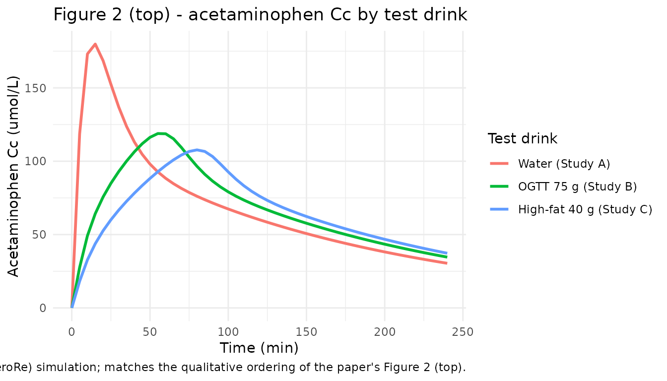
# Replicates Figure 2 (bottom): gallbladder volume time course. The
# fat-containing drink drives a substantial gallbladder ejection; the
# OGTT drink drives a small ejection; water leaves the volume at
# baseline.
ggplot(sim, aes(time, GVol, colour = cohort)) +
  geom_line(linewidth = 1) +
  labs(x = "Time (min)",
       y = "Gallbladder volume (mL)",
       colour = "Test drink",
       title = "Figure 2 (bottom) - gallbladder volume by test drink",
       caption = "Typical-value (zeroRe) simulation.") +
  theme_minimal()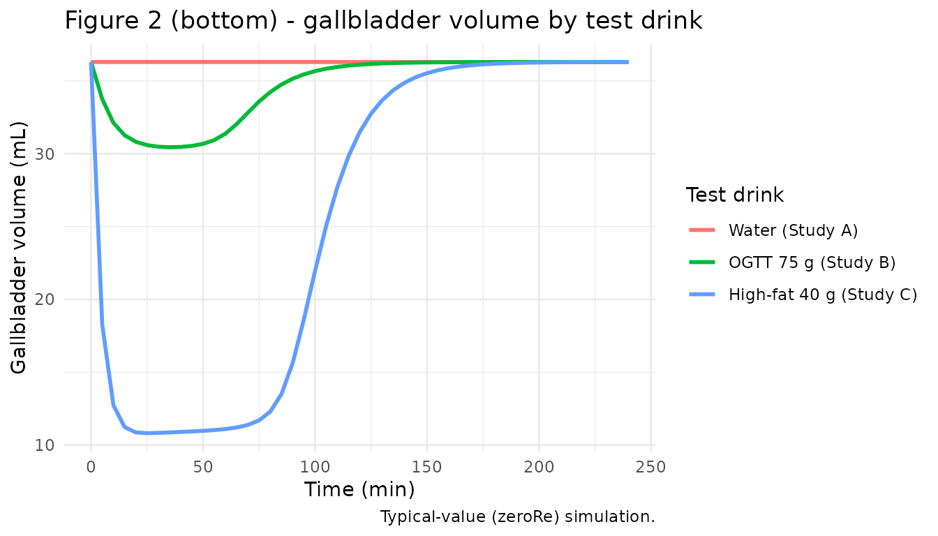
# Total plasma CCK time course (paper Supplementary Material S3). The
# high-fat drink drives the largest postprandial CCK rise via the
# duodenal Emax stimulus; the OGTT drink drives a small rise; water
# stays at baseline.
ggplot(sim, aes(time, TCCK, colour = cohort)) +
  geom_line(linewidth = 1) +
  labs(x = "Time (min)",
       y = "Total plasma CCK (pmol/L)",
       colour = "Test drink",
       title = "Postprandial total CCK by test drink",
       caption = "Typical-value (zeroRe) simulation.") +
  theme_minimal()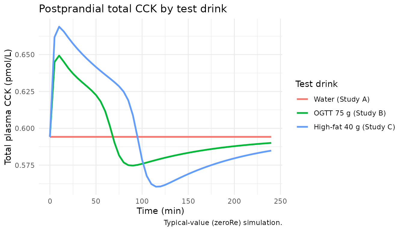
PKNCA validation
PKNCA on the acetaminophen Cc, stratified by test drink. The CCK and gallbladder volume outputs are not standard NCA targets (they describe mechanistic responses rather than drug PK), and the paper’s preferred summaries for them - time-to-50%-gastric-emptying TGE50 and gallbladder ejection fraction EF% - are reported separately in the next section.
nca_data <- sim |>
  dplyr::filter(!is.na(Cc)) |>
  dplyr::transmute(id = cohort, time, Cc)
dose_data <- sim |>
  dplyr::filter(time == 0) |>
  dplyr::distinct(cohort, .keep_all = TRUE) |>
  dplyr::transmute(id = cohort, time = 0, amt = 1500)

conc_obj <- PKNCA::PKNCAconc(nca_data, Cc ~ time | id)
dose_obj <- PKNCA::PKNCAdose(dose_data, amt ~ time | id)
intervals <- data.frame(start = 0, end = 240,
                        cmax = TRUE, tmax = TRUE,
                        auclast = TRUE, half.life = TRUE)
nca_res <- PKNCA::pk.nca(PKNCA::PKNCAdata(conc_obj, dose_obj, intervals = intervals))
knitr::kable(summary(nca_res),
caption = "Acetaminophen NCA (simulated typical-value, by test drink).")| start | end | N | auclast | cmax | tmax | half.life |
|---|---|---|---|---|---|---|
| 0 | 240 | 3 | 16500 [3.60] | 132 [27.7] | 55.0 [15.0, 80.0] | 121 [0.112] |
Derived summaries: TGE50 and gallbladder ejection fraction
The paper’s preferred mechanistic summaries are the time to empty 50% of the stomach content (TGE50) and the gallbladder ejection fraction (EF%, Eq. 1 of the paper). These quantities derive from the simulated trajectories rather than from NCA.
# TGE50 derived from the stomach acetaminophen amount (the per-cohort
# initial dose is 1500 mg into the stomach; the trajectory falls
# monotonically until KG drains it past 50% of the initial value).
tge50 <- sim |>
  group_by(cohort) |>
  summarise(
    initial_stomach = max(stomach, na.rm = TRUE),
    tge50_min       = approx(stomach / max(stomach), time,
                             xout = 0.5)$y,
    .groups         = "drop"
  )
knitr::kable(tge50,
caption = "Time to empty 50% of the stomach content (TGE50, min).")| cohort | initial_stomach | tge50_min |
|---|---|---|
| Water (Study A) | 1500 | 2.512542 |
| OGTT 75 g (Study B) | 1500 | 20.941369 |
| High-fat 40 g (Study C) | 1500 | 33.733577 |
ef_pct <- sim |>
  group_by(cohort) |>
  summarise(
    base_volume = first(GVol),
    min_volume  = min(GVol, na.rm = TRUE),
    ef_pct      = 100 * (first(GVol) - min(GVol, na.rm = TRUE)) /
                  first(GVol),
    .groups     = "drop"
  )
knitr::kable(ef_pct,
caption = "Gallbladder ejection fraction (EF%, Eq. 1 of the paper).")| cohort | base_volume | min_volume | ef_pct |
|---|---|---|---|
| Water (Study A) | 36.3 | 36.30000 | 0.00000 |
| OGTT 75 g (Study B) | 36.3 | 30.44866 | 16.11939 |
| High-fat 40 g (Study C) | 36.3 | 10.81284 | 70.21256 |
The paper reports a simulation-based TGE50 of 3.8 min (PI95 0.2-15) for water and up to 96 min (PI95 64-133) for a high-fat drink, with gallbladder ejection fraction up to 65% (PI95 37-82) for the high-fat drink (Results). The typical-value simulation above falls within these prediction-interval envelopes for the three test drinks shown.
Assumptions and deviations
- Joint-model topology - parallel nutrient tracks. Figure 1 of the paper shows three separate first-order rate constants for nutrient disappearance: KUL (from the “upper SI”, driving the GE feedback), KDJ (from the “duodenum”, driving CCKF and GBE), and KJI (from the “upper jejunum”, driving CCKL). All three are reported as separate parameters in Table 3 (KUL estimated in the GE column; KDJ and KJI fixed from Hens 2008 and shared between the CCK and GBE columns). The literal reading of Figure 1 + Table 3 is therefore that the joint model carries three parallel nutrient signal tracks downstream of the stomach - an upper-SI track (drains via KUL) for the GE caloric feedback, and a duodenum-then-upper-jejunum chain (drains via KDJ then KJI) for the CCK and GBE signals. This is what the packaged model implements: each per-macronutrient stomach state feeds both downstream tracks simultaneously, with the same KG rate exit. Mass is not strictly conserved across the parallel tracks (each track is a delayed signal representation of the stomach content rather than a physical mass-balance compartment). The alternative interpretation - a single chain stomach -> duodenum -> upper jejunum with the GE feedback reading the lumped duodenum + upper jejunum content - cannot be ruled out without the Supplementary Material S1 (NONMEM control code), which is not on disk in this worktree and not retrievable from open-access mirrors. Operators who can access S1 are encouraged to confirm the topology choice and (if warranted) refit the model into a single-chain form; the parameter estimates from Table 3 carry over directly under either topology.
- Covariate-effect reference values. The WT-BASEBILE (+1.19%/kg) and AGE-S50_BILE (+2.15%/yr) effects are linear-deviation forms that require a reference value (WT_ref, AGE_ref) for the deviation to be zero. The paper reports the effect coefficients in Table 3 but does not state the reference values explicitly; the natural NONMEM default is the population mean / median, which from Table 1 of the paper is approximately WT = 88 kg and AGE = 58 y across the pooled Studies A-C. The Supplementary Material S1 control stream would disambiguate the reference values; if S1 is later inspected, re-fitting the typical-value BASEBILE and S50_BILE may be required to keep the cohort-mean predictions aligned with the paper.
-
SLPCAL parameterisation. SLPCAL is a negative slope
on the linear-scale gastric-emptying feedback (-0.0173 /kcal in Table
3). The packaged model encodes |SLPCAL| as
exp(lslpcal_mag)so the reported 19% CV between-subject variability can be carried as a standard log-normal eta on the magnitude (with the sign fixed negative inmodel()). This is equivalent to the NONMEM idiomSLPCAL_i = -THETA(SLPCAL) * exp(ETA(SLPCAL))and preserves the paper’s interpretation that the caloric feedback is always inhibitory of GE. -
GE-onset gating for water. The paper reports that
no onset delay was needed for the Study A water arm. The packaged model
implements this as
onset = 1forDRINK_OGTT = DRINK_FAT = 0(a branch in the modelonsetexpression that adds back to 1 when both binary indicators are zero), so simulating water reproduces the paper’s immediate-onset behaviour without further parameter changes. -
TAD via raw model time. The Hill onset function
uses time after dose. Because the study protocol co-administers the test
drink and acetaminophen at t = 0 (an oral dose for Studies B-D, a 1-min
nasogastric infusion for Study A), the packaged model uses the raw model
time variable t as a stand-in for TAD. Downstream users dosing at a
nonzero time should shift the data so t = 0 corresponds to the dose
time, or modify the model to use the rxode2
tad()function with a registered dose compartment. -
IPPSE coupling not simulated. The paper used an
individual pharmacokinetic-parameters-with-standard-errors (IPPSE)
approach in which the per-subject KG estimates from the GE submodel fit
were carried into the CCK and GBE submodel fits. In simulation from the
packaged model, KG is sampled from the population distribution (BSV 155%
CV via
etalkg0) and is therefore not perfectly individualised to the simulated subject’s nutrient amounts. This is a standard simplification when a single joint model is simulated forward; the typical-value predictions are unaffected. - Supplementary Material S2 (parameter shrinkages) not on disk. The paper’s S2 reports shrinkage diagnostics for the etas; these are not parameter values that drive the simulation but help interpret the realism of the BSV distributions. They are not embedded in the packaged model.
- Acetaminophen molecular weight 151.17 g/mol. The paracetamol-amount-to-uM (= umol/L) conversion uses the standard IUPAC molecular weight; the paper does not report the conversion constant explicitly.