How do I...?

Short answers to common tasks. Each recipe is a few lines of code with a link to the page that explains it in full.

All recipes use this one-compartment oral model with between-subject variability and proportional residual error:

library(rxode2)
#> rxode2 5.1.8.9000 using 2 threads (see ?getRxThreads)
#>   no cache: create with `rxCreateCache()`

mod <- function() {
  ini({
    tka <- log(1.15)
    tcl <- log(0.135)
    tv <- log(8)
    eta.ka ~ 0.6
    eta.cl ~ 0.3
    eta.v ~ 0.1
    prop.sd <- 0.1
  })
  model({
    ka <- exp(tka + eta.ka)
    cl <- exp(tcl + eta.cl)
    v <- exp(tv + eta.v)
    d/dt(depot) <- -ka * depot
    d/dt(center) <- ka * depot - cl / v * center
    cp <- center / v
    cp ~ prop(prop.sd)
  })
}

Dosing

…give a dose every 12 hours for a week?

ev <- et(amt = 300, ii = 12, until = 168) |>
  et(seq(0, 168, by = 1))
s <- rxSolve(mod, ev)
#> ℹ parameter labels from comments are typically ignored in non-interactive mode
#> ℹ Need to run with the source intact to parse comments
plot(s, cp)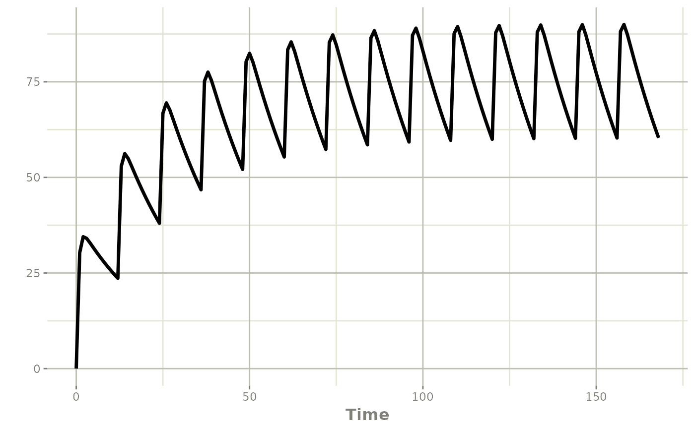

More: Building event tables with et().

…give a loading dose followed by maintenance doses?

ev <- et(amt = 600) |>
  et(time = 12, amt = 300, ii = 12, until = 168) |>
  et(seq(0, 168, by = 1))

More: Combining event tables.

…give an infusion?

Give the duration with dur (or the rate with rate), dosing into the central compartment:

ev <- et(amt = 300, dur = 2, cmt = "center") |>
  et(seq(0, 24, by = 0.5))

More: Dosing event types.

…start at steady state?

ev <- et(amt = 300, ii = 12, ss = 1) |>
  et(seq(0, 24, by = 0.5))

More: Dosing event types.

…use my own NONMEM-style dataset?

Pass the data frame straight to rxSolve(); columns are matched by name (ID, TIME, AMT, EVID, CMT, …):

d <- data.frame(ID = 1, TIME = c(0, 1, 2, 4, 8, 12),
                AMT = c(300, 0, 0, 0, 0, 0), EVID = c(1, 0, 0, 0, 0, 0),
                CMT = c("depot", rep("center", 5)))
s <- rxSolve(mod, d)

More: Dataset columns.

…dose based on the current model state?

Use bolus(), infuse() and friends inside model().

More: Dosing from inside the model.

Simulation

…simulate the typical individual (no variability)?

ev <- et(amt = 300, ii = 12, until = 72) |>
  et(seq(0, 72, by = 0.5))
s <- rxSolve(zeroRe(mod), ev)
#> ℹ parameter labels from comments are typically ignored in non-interactive mode
#> ℹ Need to run with the source intact to parse comments
#> ℹ omega/sigma items treated as zero: 'eta.ka', 'eta.cl', 'eta.v'

More: ?zeroRe.

…simulate a population?

s <- rxSolve(mod, ev, nSub = 100)

Each subject draws its own eta values from the ini() block. More: Simulating populations.

…get simulated observations with residual error?

The endpoint cp ~ prop(prop.sd) adds residual error; the simulated observation is in the sim column, the prediction stays in cp (subjects simulated with nSub are numbered in sim.id):

head(s[, c("sim.id", "time", "cp", "sim")])
#>   sim.id time       cp      sim
#> 1      1  0.0  0.00000  0.00000
#> 2      1  0.5 13.26744 11.65917
#> 3      1  1.0 18.49685 20.99101
#> 4      1  1.5 20.48233 19.20431
#> 5      1  2.0 21.15935 20.59761
#> 6      1  2.5 21.30931 24.39596

…make a simulation reproducible?

s1 <- rxSolve(mod, ev, nSub = 10, seed = 42)
s2 <- rxSolve(mod, ev, nSub = 10, seed = 42)
all.equal(s1$sim, s2$sim)
#> [1] TRUE

More: ?rxWithSeed.

…add parameter uncertainty?

Give a covariance matrix for the population parameters with thetaMat and the number of studies with nStud:

s <- rxSolve(mod, ev, nSub = 20, nStud = 5,
             thetaMat = lotri::lotri(tcl ~ 0.01, tv ~ 0.01))

More: Parameter uncertainty.

…summarize a simulation with prediction intervals?

s <- rxSolve(mod, ev, nSub = 200, seed = 42)
ci <- confint(s, "sim", level = 0.90)
#> ! in order to put confidence bands around the intervals, you need at least 2500 simulations
#> summarizing data...done
plot(ci)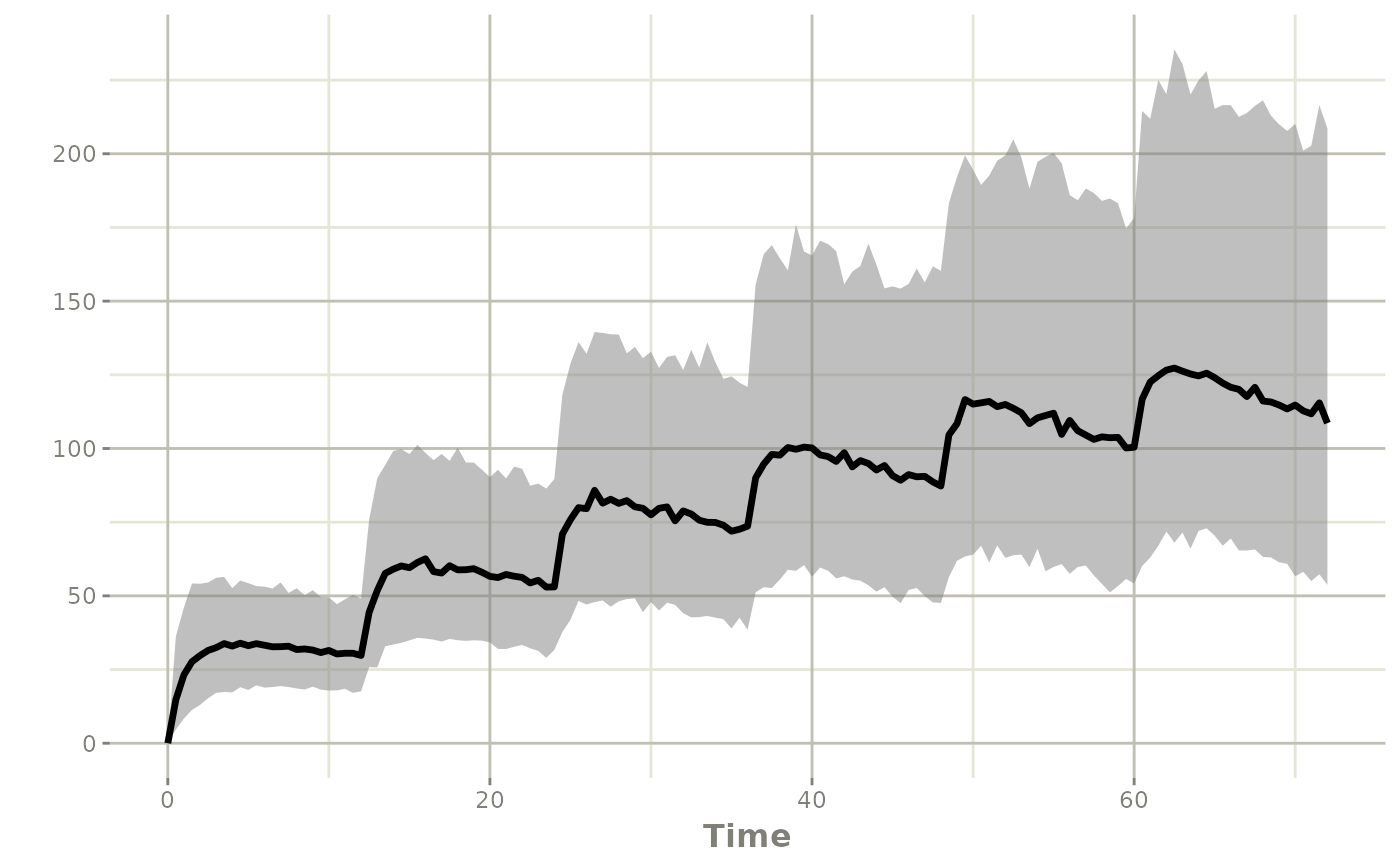

More: Summarizing simulations with confint().

…simulate between-occasion variability?

More: Nesting levels.

Covariates

…add a covariate effect?

Pipe a new line into the model; the covariate WT becomes an input:

modWt <- mod |>
  model(cl <- exp(tcl + eta.cl) * (WT / 70)^0.75)
#> ℹ parameter labels from comments are typically ignored in non-interactive mode
#> ℹ Need to run with the source intact to parse comments
#> ℹ add covariate `WT`

More: Modifying models.

…give each subject their own covariate value?

s <- rxSolve(modWt, ev,
             iCov = data.frame(id = 1:4, WT = c(50, 70, 90, 110)))

More: Covariates.

…use a covariate that changes over time?

Add it as a column of the data; values are interpolated between rows:

d <- as.data.frame(et(amt = 300, ii = 24, until = 96) |>
                     et(seq(0, 96, by = 4)))
d$WT <- 70 - d$time / 24
s <- rxSolve(modWt, d)

More: Covariates.

Output and speed

…get output only at specific times?

ev <- et(amt = 300) |> et(c(0.5, 1, 2, 4, 8, 12, 24))
rxSolve(zeroRe(mod), ev)
#> ℹ parameter labels from comments are typically ignored in non-interactive mode
#> ℹ Need to run with the source intact to parse comments
#> ℹ omega/sigma items treated as zero: 'eta.ka', 'eta.cl', 'eta.v'
#> ── Solved rxode2 object ──
#> ── Parameters (x$params): ──
#>        tka        tcl         tv    prop.sd     eta.ka     eta.cl      eta.v 
#>  0.1397619 -2.0024805  2.0794415  0.0000000  0.0000000  0.0000000  0.0000000 
#> ── Initial Conditions (x$inits): ──
#>  depot center 
#>      0      0 
#> ── First part of data (object): ──
#> # A tibble: 7 × 9
#>    time    ka    cl     v    cp ipredSim   sim      depot center
#>   <dbl> <dbl> <dbl> <dbl> <dbl>    <dbl> <dbl>      <dbl>  <dbl>
#> 1   0.5  1.15 0.135  8.00  16.3     16.3  16.3 169.         131.
#> 2   1    1.15 0.135  8.00  25.4     25.4  25.4  95.0        203.
#> 3   2    1.15 0.135  8.00  33.0     33.0  33.0  30.1        264.
#> 4   4    1.15 0.135  8.00  35.2     35.2  35.2   3.02       282.
#> 5   8    1.15 0.135  8.00  33.2     33.2  33.2   0.0303     266.
#> 6  12    1.15 0.135  8.00  31.1     31.1  31.1   0.000305   249.
#> # ℹ 1 more row

…keep input columns in the output?

d$GROUP <- "A"
s <- rxSolve(modWt, d, keep = c("WT", "GROUP"))
head(s[, c("time", "cp", "WT", "GROUP")])
#>   time       cp       WT GROUP
#> 1    0  0.00000 70.00000     A
#> 2    4 55.13529 69.83333     A
#> 3    8 52.49335 69.66667     A
#> 4   12 49.23268 69.50000     A
#> 5   16 46.16918 69.33333     A
#> 6   20 43.30109 69.16667     A

…plot the result?

plot(s, cp)

More: Plotting.

…solve faster?

Use more threads for multi-subject problems:

s <- rxSolve(mod, ev, nSub = 100, cores = 2)

More: Speeding up solving.

…solve a population too large for memory?

More: Out-of-memory solving.

Models

…change an initial estimate or fix a parameter?

mod2 <- mod |> ini(tcl = log(0.2))
#> ℹ parameter labels from comments are typically ignored in non-interactive mode
#> ℹ Need to run with the source intact to parse comments
#> ℹ change initial estimate of `tcl` to `-1.6094379124341`
mod3 <- mod |> ini(tv = fix)
#> ℹ parameter labels from comments are typically ignored in non-interactive mode
#> ℹ Need to run with the source intact to parse comments
#> ℹ fix `tv` to `2.07944154167984`