Dual Absorption Models with splitBolus()

2026-05-23

Background

Some drugs exhibit two distinct absorption phases after oral dosing. A classic example is a modified-release tablet where an immediate-release coat dissolves rapidly in the stomach while a matrix core releases drug more slowly in the intestine. Another example is a drug with meaningful gastric absorption in addition to the usual intestinal absorption. Either way, the plasma concentration versus time profile shows a secondary rise or shoulder that a simple first-order depot model cannot capture.

The traditional workaround is to split the dose in the dataset: add a second row with the same dose time but directed at a different compartment, and scale each row’s amount by the fraction going through each pathway. This ties the model structure to the data format and forces dataset edits whenever the model changes.

splitBolus() is a model-only directive in rxode2 that moves this split into the model block. Bolus doses arriving at the source compartment are transparently redirected to one or more target compartments. The dataset never changes.

Setup: a shared oral-dosing event table

library(rxode2)

ev <- et(amt = 100, time = 0, cmt = "depot", ii = 24, addl = 6) |>
  et(seq(0, 168, by = 1))

This event table represents a week of once-daily 100 mg oral doses with hourly observations. Both models below will use ev unchanged.

Single first-order absorption model

First to show we start with a single one-compartment oral absorption model:

modSingle <- function() {
  ini({
    tka <- log(1.2)
    tcl <- log(6)
    tv  <- log(40)
  })
  model({
    ka <- exp(tka)
    cl <- exp(tcl)
    v  <- exp(tv)
    d/dt(depot)   <- -ka * depot
    d/dt(central) <- ka * depot - cl / v * central
    cp <- central / v
  })
}

resSingle <- rxSolve(modSingle, ev)
plot(resSingle, cp)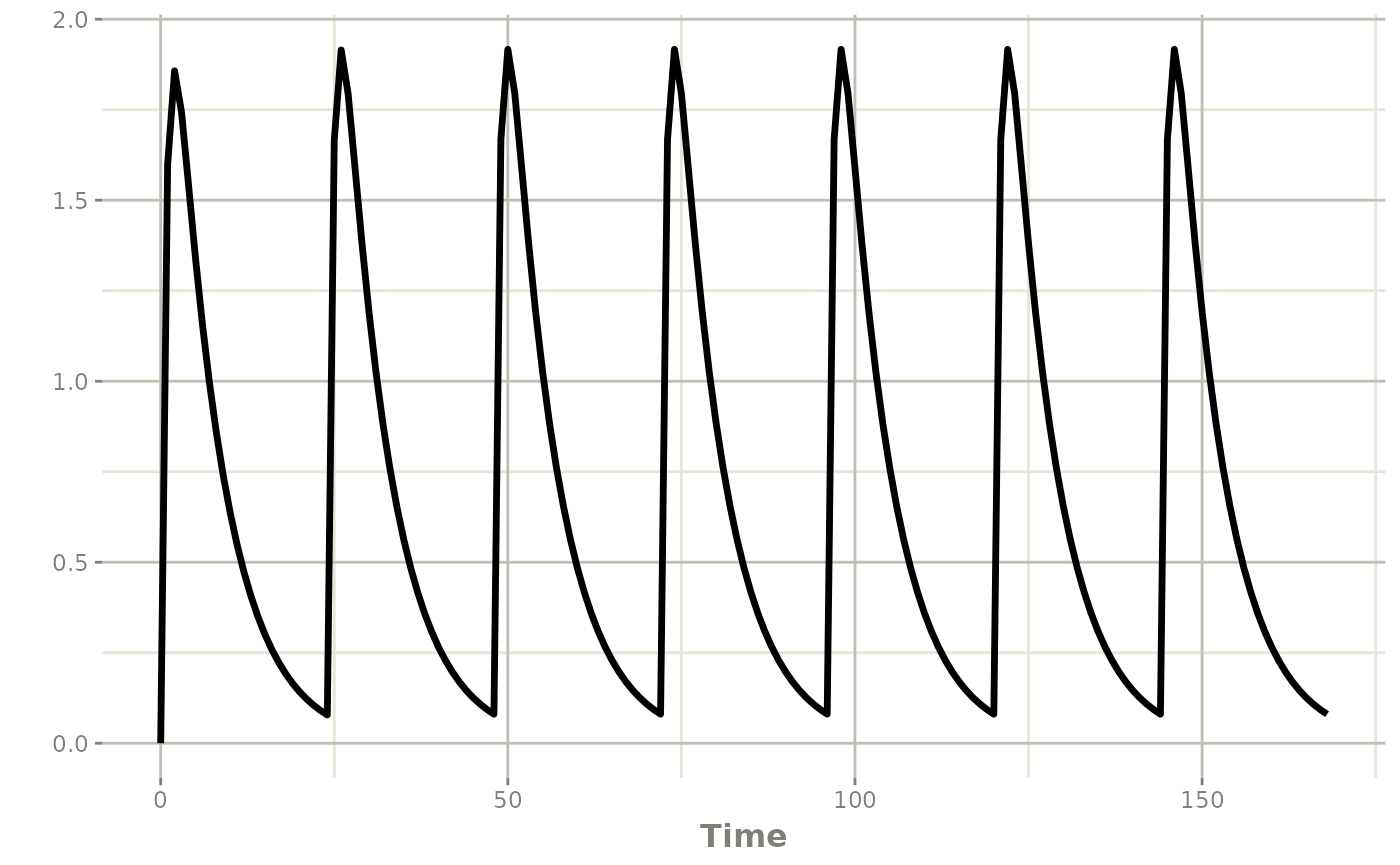

Dual absorption model with splitBolus

To add a second absorption pathway, we change only the model. The event table ev stays exactly the same.

splitBolus(depot, depot, depotSlow) tells rxode2 that any bolus dose directed at depot should instead be applied to depot and depotSlow. Both target compartments receive the full original amount, so bioavailability modifiers f(depot) and f(depotSlow) are used to partition the dose between the two pathways; The lag(depotSlow) is to show how much time the second part of the dose started to release.

modDual <- function() {
  ini({
    tka1 <- log(0.4)
    tka2 <- log(0.2)
    fa   <- 0.7
    tcl  <- log(6)
    tv   <- log(40)
  })
  model({
    ka1 <- exp(tka1)
    ka2 <- exp(tka2)
    cl  <- exp(tcl)
    v   <- exp(tv)

    splitBolus(depot, depot, depotSlow)
    f(depot) <- fa
    f(depotSlow) <- 1 - fa
    lag(depotSlow) <- 6

    d/dt(depot) <- -ka1 * depot
    d/dt(depotSlow) <- -ka2 * depotSlow
    d/dt(central)   <- ka1 * depot + ka2 * depotSlow - cl / v * central
    cp <- central / v
  })
}

resDual <- rxSolve(modDual, ev)
plot(resDual, cp)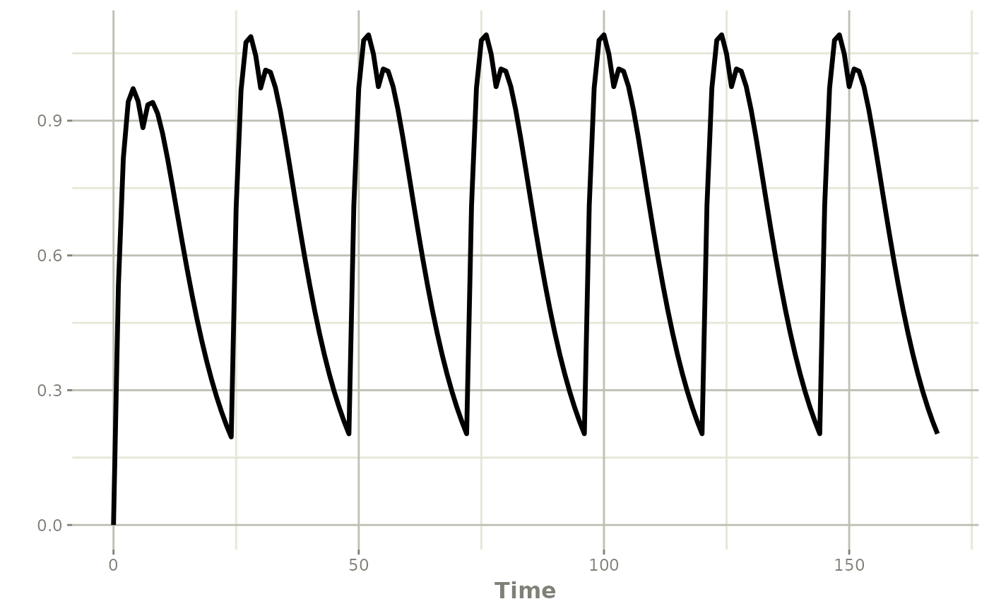

The parameters here are:

Parameter	Meaning
tka1	Log of the fast absorption rate constant (hr⁻¹)
tka2	Log of the slow absorption rate constant (hr⁻¹)
fa	Fraction of the dose entering the fast pathway
tcl	Log of clearance (L/hr)
tv	Log of central volume (L)

Comparing the two concentration profiles

library(ggplot2)

dfSingle <- as.data.frame(resSingle)[, c("time", "cp")]
dfSingle$model <- "Single absorption"

dfDual <- as.data.frame(resDual)[, c("time", "cp")]
dfDual$model <- "Dual absorption"

dfAll <- rbind(dfSingle, dfDual)

ggplot(dfAll, aes(time, cp, color = model)) +
  geom_line() +
  labs(x = "Time (hr)", y = "Concentration (mg/L)", color = NULL) +
  theme_bw()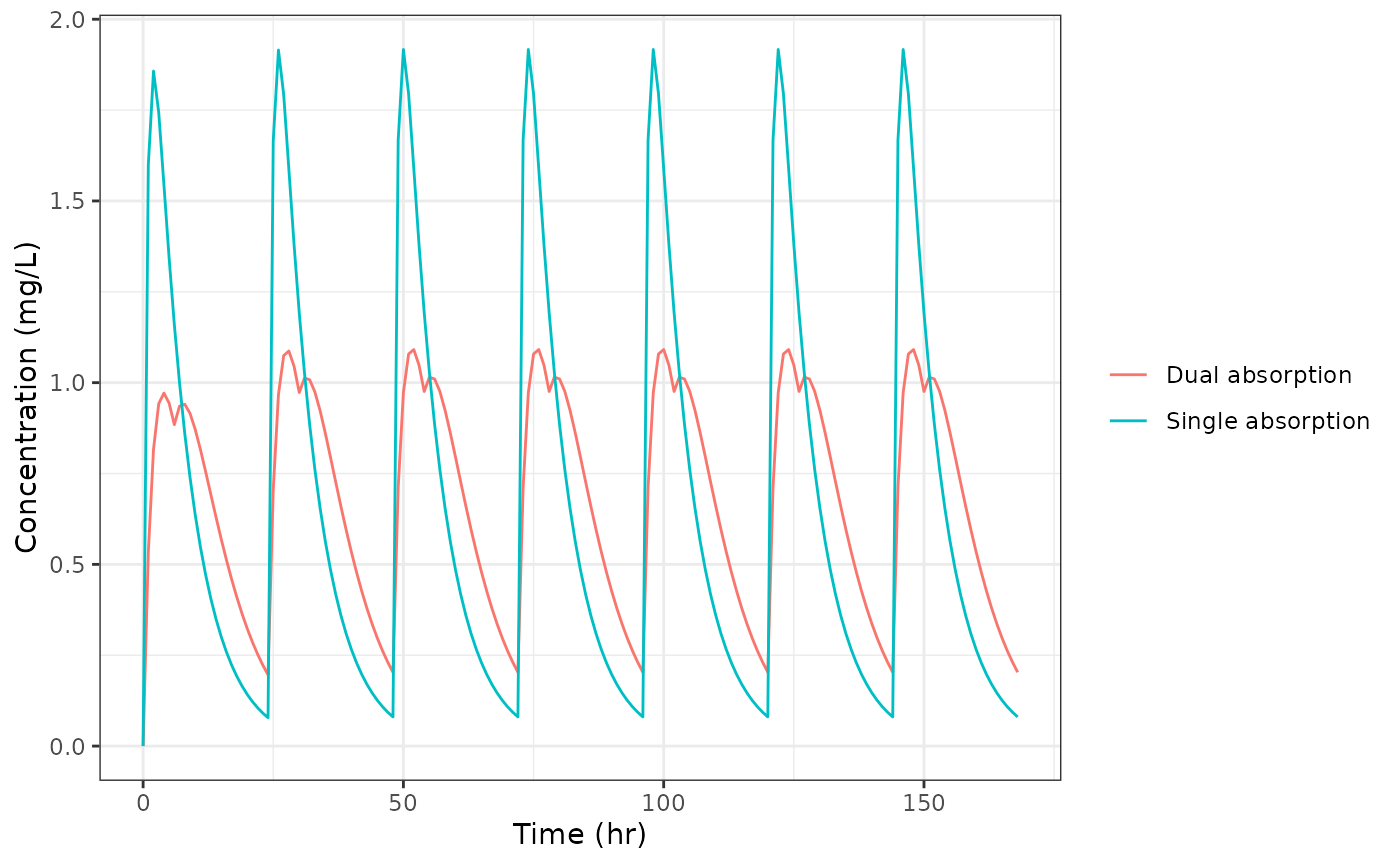

The dual absorption profile shows a shoulder on the ascending limb of each dose interval, driven by the slow pathway continuing to deliver drug after the fast pathway has been nearly exhausted.

Key points

• The event table ev is identical for both models. No dataset edits are needed to switch from single to dual absorption.

• splitBolus(depot, depot, depotSlow) intercepts every bolus arriving at depot and redirects it to depot and depotSlow. The source compartment depot itself never accumulates drug.

• f(depot) <- fa and f(depotSlow) <- 1 - fa ensure the dose is partitioned so that the total amount absorbed equals the original dose (when fa is between 0 and 1).

• The same approach scales to population simulations: supply an iCov or omega matrix to rxSolve() and the dataset requires no changes.

• More than two pathways are possible-simply list additional target compartments in splitBolus() and add corresponding f() modifiers.