Clinical Trial Simulation with rxode2
Source:vignettes/articles/rxode2-clinical-trial-sim.Rmd
rxode2-clinical-trial-sim.Rmd
library(rxode2)
#> rxode2 5.1.3 using 2 threads (see ?getRxThreads)
#>   no cache: create with `rxCreateCache()`
library(ggplot2)
library(data.table)
#>
#> Attaching package: 'data.table'
#> The following object is masked from 'package:base':
#>
#>     %notin%
Overview
Clinical trial simulation (CTS) uses a pharmacometric model to predict trial outcomes in silico before running an expensive study. Common applications include:
- Dose regimen selection – which dose and frequency optimizes exposure relative to a PK/PD target?
- Target attainment analysis (TAA) – what fraction of patients achieves the desired exposure target?
- Sample-size estimation by simulation – how many subjects are needed to detect a treatment difference with adequate power?
- Special population predictions – paediatric, renal impairment, or other covariate subgroups.
Model setup
We use a one-compartment oral PK model linked to a simple Emax PD model to illustrate several CTS tasks.
pkpdModel <- function() {
  ini({
    tka   <- log(1.0);  label("log Ka (1/h)")
    tcl   <- log(0.5);  label("log CL (L/h)")
    tv    <- log(5.0);  label("log V (L)")
    temax <- log(80);   label("log Emax (%)")
    tec50 <- log(2.0);  label("log EC50 (mg/L)")
    eta.cl ~ 0.09
    eta.v  ~ 0.09
    prop.sd <- 0.15
  })
  model({
    ka   <- exp(tka)
    cl   <- exp(tcl + eta.cl)
    v    <- exp(tv  + eta.v)
    emax <- exp(temax)
    ec50 <- exp(tec50)
    d/dt(depot)  <- -ka * depot
    d/dt(center) <- ka * depot - cl / v * center
    cp   <- center / v
    ## Emax PD model
    effect <- emax * cp / (ec50 + cp)
    cp ~ prop(prop.sd)
  })
}
Dose regimen comparison
Compare three once-daily oral doses (50, 100, 200 mg) in a 1000-subject population.
nSub  <- 1000
doses <- c(50, 100, 200)

# Build a list of event tables -- one per dose
evList <- lapply(doses, function(d) {
  et(amt = d, ii = 24, addl = 6) |>   # 7-day QD
    et(seq(0, 168, by = 1))            # hourly observations
})

# Simulate all doses in one call using a named list
simList <- lapply(seq_along(doses), function(i) {
  res <- rxSolve(pkpdModel, evList[[i]], nSub = nSub,
                 returnType = "data.frame")
  res$dose <- doses[i]
  res
})

simAll <- rbindlist(simList)
Concentration-time profiles by dose
dt <- as.data.table(simAll)

medCI <- dt[, .(
  p05 = quantile(cp, 0.05),
  p50 = quantile(cp, 0.50),
  p95 = quantile(cp, 0.95)
), by = .(time, dose)]

ggplot(medCI, aes(x = time, group = factor(dose), colour = factor(dose),
                  fill = factor(dose))) +
  geom_ribbon(aes(ymin = p05, ymax = p95), alpha = 0.15, colour = NA) +
  geom_line(aes(y = p50), linewidth = 1) +
  labs(x = "Time (h)", y = "Concentration (mg/L)",
       colour = "Dose (mg)", fill = "Dose (mg)",
       title = "Dose comparison -- steady-state concentration profiles") +
  theme_bw()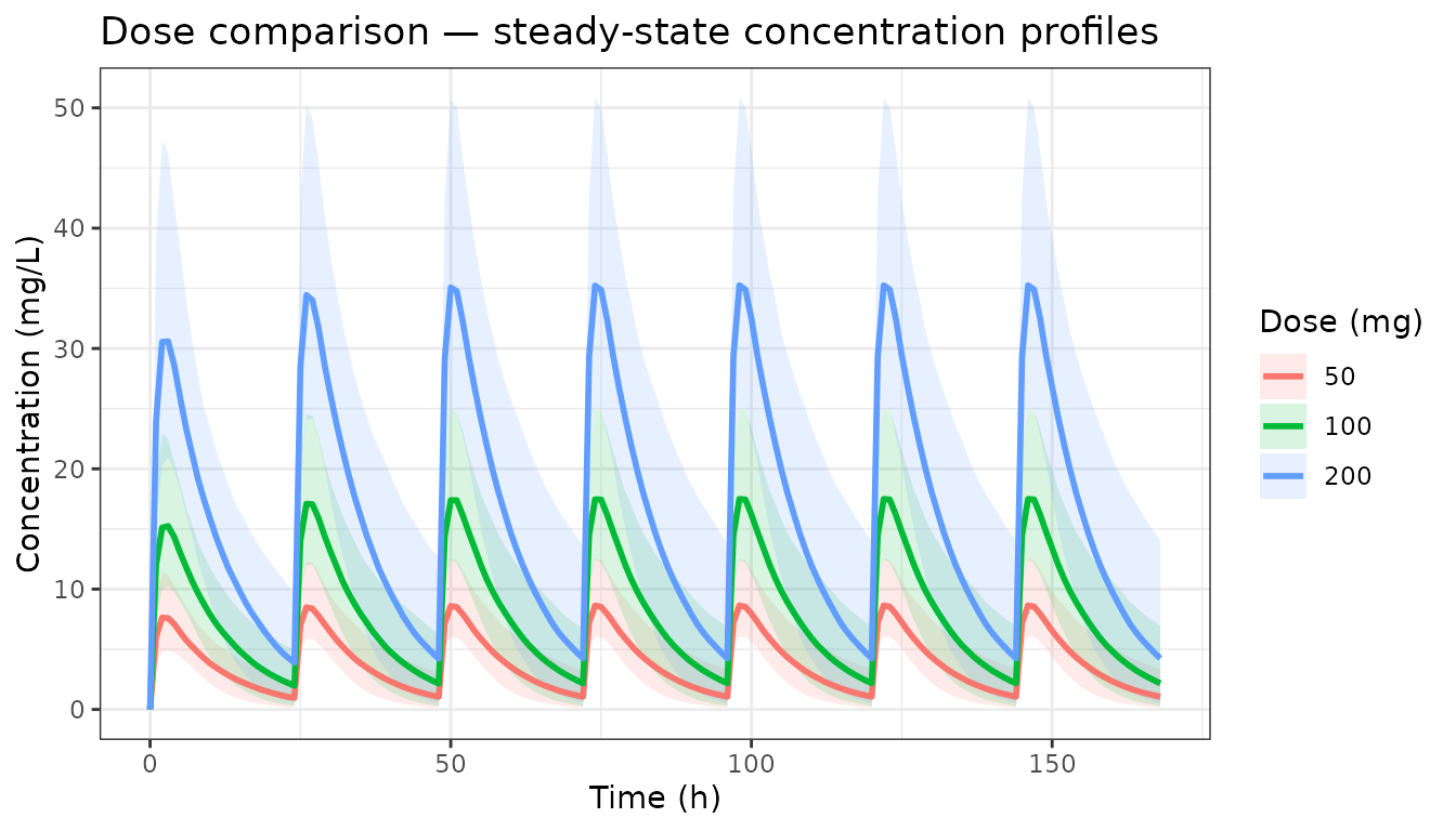
Target attainment analysis (TAA)
Define a PK target as trough concentration >= 1 mg/L at steady state (day 7, trough = 168 h).
trough <- dt[time == 168, .(
  pctAbove = mean(cp >= 1.0) * 100
), by = dose]

ggplot(trough, aes(x = factor(dose), y = pctAbove)) +
  geom_col(fill = "steelblue", width = 0.5) +
  geom_hline(yintercept = 90, linetype = "dashed", colour = "red") +
  labs(x = "Dose (mg)", y = "% subjects with trough >= 1 mg/L",
       title = "Target attainment at steady-state trough",
       subtitle = "Dashed line: 90% target attainment criterion") +
  theme_bw()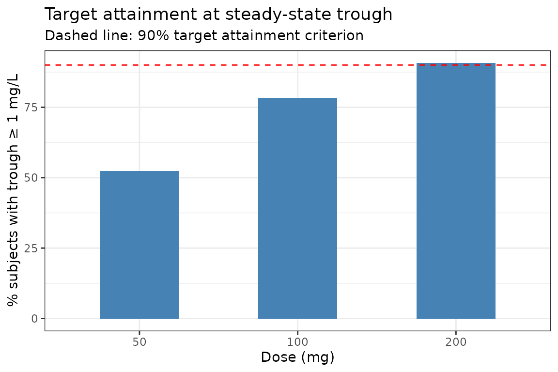
PK/PD target: % of population with effect >= 50%
Using the Emax model, what fraction achieves >= 30% of maximum effect at the trough?
pdTarget <- dt[time == 168, .(
  pctTarget = mean(effect >= 30) * 100
), by = dose]

ggplot(pdTarget, aes(x = factor(dose), y = pctTarget)) +
  geom_col(fill = "coral", width = 0.5) +
  geom_hline(yintercept = 80, linetype = "dashed", colour = "red") +
  labs(x = "Dose (mg)", y = "% subjects with effect >= 30%",
       title = "PD target attainment at steady-state trough",
       subtitle = "Dashed line: 80% target attainment criterion") +
  theme_bw()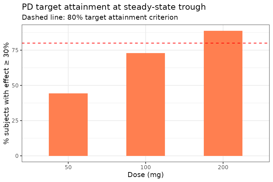
Exposure metric distributions
Compute AUC over one dosing interval at steady state (day 7, hours 144-168) for each dose.
ss <- dt[time >= 144 & time <= 168]

aucSS <- ss[, .(
  AUCtau = sum(diff(time) * (cp[-length(cp)] + cp[-1]) / 2)
), by = .(sim.id, dose)]

ggplot(aucSS, aes(x = AUCtau, fill = factor(dose))) +
  geom_density(alpha = 0.4) +
  labs(x = "AUC_tau (mg.h/L)", y = "Density",
       fill = "Dose (mg)",
       title = "Steady-state AUC_tau distribution by dose") +
  theme_bw()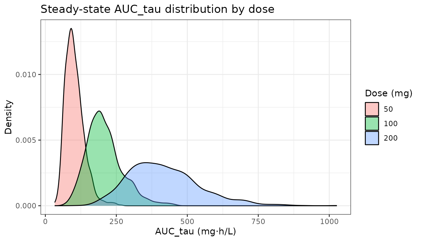
Sample-size estimation by simulation
Estimate the power to detect a difference in mean trough concentration between 100 mg and 50 mg using a two-sample t-test, as a function of sample size.
set.seed(99)
nSizes  <- c(5, 10, 15, 20, 30)
nTrials <- 200   # increase to >= 1000 for stable power estimates

powerRes <- rbindlist(lapply(nSizes, function(n) {
  pvals <- vapply(seq_len(nTrials), function(trial) {
    # Simulate n subjects per arm
    sim50  <- rxSolve(pkpdModel,
                      et(amt = 50,  ii = 24, addl = 6) |> et(168),
                      nSub = n, returnType = "data.frame")
    sim100 <- rxSolve(pkpdModel,
                      et(amt = 100, ii = 24, addl = 6) |> et(168),
                      nSub = n, returnType = "data.frame")
    t.test(sim100$cp, sim50$cp)$p.value
  }, numeric(1))
  data.table(n = n, power = mean(pvals < 0.05))
}))
ggplot(powerRes, aes(x = n, y = power)) +
  geom_line(linewidth = 1, colour = "steelblue") +
  geom_point(size = 2) +
  geom_hline(yintercept = 0.80, linetype = "dashed", colour = "red") +
  scale_y_continuous(labels = scales::percent, limits = c(0, 1)) +
  labs(x = "Subjects per arm", y = "Power",
       title = "Power by simulation -- 100 mg vs 50 mg trough comparison",
       subtitle = "Dashed line: 80% power target. ~23 subjects/arm sufficient here.") +
  theme_bw()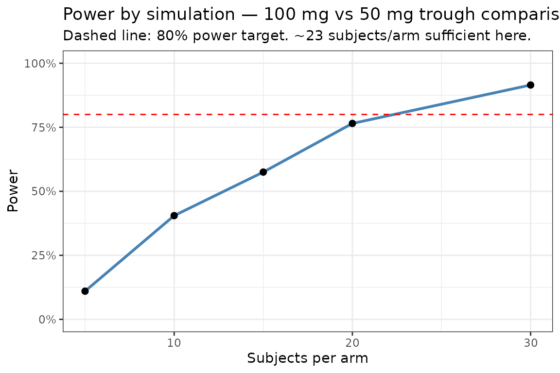
Special population simulation
Simulate the 100 mg dose in a paediatric population with lower body weight driving CL allometrically:
# Covariate table for a paediatric cohort (n=200, WT 10-40 kg)
set.seed(7)
pedCovs <- data.frame(
  id = 1:200,
  WT = runif(200, 10, 40)
)

# Model with allometric CL scaling
pedModel <- pkpdModel |>
  model({
    cl <- exp(tcl + eta.cl) * (WT / 70)^0.75
    v  <- exp(tv  + eta.v)  * (WT / 70)
  }, append = NA)

pedSim <- rxSolve(
  pedModel,
  et(amt = 100, ii = 24, addl = 6) |>
    et(seq(0, 168, by = 2)) |>
    et(id=1:200),
  iCov = pedCovs,
  nSub = nrow(pedCovs),
  returnType = "data.frame"
)

pedDT <- as.data.table(pedSim)
pedCI <- pedDT[, .(p05 = quantile(cp, 0.05),
                   p50 = quantile(cp, 0.50),
                   p95 = quantile(cp, 0.95)), by = time]

ggplot(pedCI, aes(x = time)) +
  geom_ribbon(aes(ymin = p05, ymax = p95), fill = "coral", alpha = 0.3) +
  geom_line(aes(y = p50), colour = "coral", linewidth = 1) +
  labs(x = "Time (h)", y = "Concentration (mg/L)",
       title = "Paediatric simulation -- 100 mg QD with allometric scaling",
       subtitle = "WT range 10-40 kg") +
  theme_bw()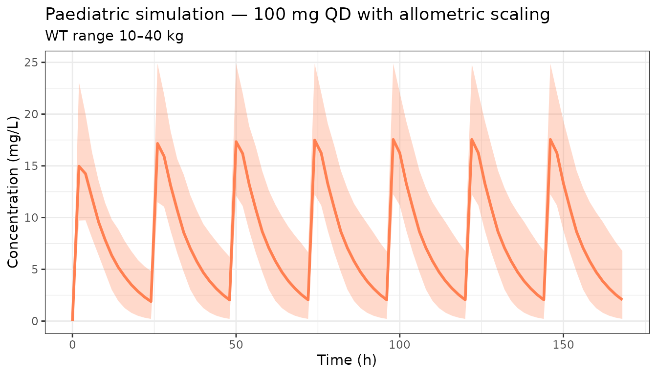
Tips
- Use
rxSetSeed()/rxWithSeed()for reproducible simulations. - Increase
nSubandnTrials(for power simulations) for production analyses; the values used here are kept small for build speed. - Combine parameter uncertainty (see the parameter uncertainty vignette) with BSV for the most complete uncertainty propagation.
- The
nlmixr2libpackage provides published models ready for use in clinical trial simulations.