library(rxode2)
#> rxode2 5.1.3 using 2 threads (see ?getRxThreads)
#>   no cache: create with `rxCreateCache()`
library(ggplot2)
What is a VPC?
A visual predictive check (VPC) is a simulation-based diagnostic that compares the distribution of observed data to the distribution of model-predicted data. The observed data are overlaid on prediction intervals (e.g. 5th, 50th, 95th percentiles) computed from many simulated replicates of the study design. A well-fitting model produces prediction intervals that envelop the observed percentiles.
Setting up the model and observed data
We use a two-compartment PK model estimated from the
theo_sd dataset (single-dose theophylline) to illustrate
the workflow.
pkModel <- function() {
  ini({
    tka  <- log(1.57)
    tcl  <- log(2.72)
    tv   <- log(31.07)
    eta.ka ~ 0.6
    eta.cl ~ 0.09
    eta.v  ~ 0.1
    add.sd <- 0.7
  })
  model({
    ka  <- exp(tka + eta.ka)
    cl  <- exp(tcl + eta.cl)
    v   <- exp(tv  + eta.v)
    d/dt(depot) <- -ka * depot
    d/dt(center) <- ka * depot - cl / v * center
    cp  <- center / v
    cp  ~ add(add.sd)
  })
}
For illustration we use the built-in theo_sd dataset as
observed data:
obs <- nlmixr2data::theo_sdNote these may come from many sources, a native nlmixr2
model, or an imported model from another tool like NONMEM or
Monolix.
Running replicated simulations
A VPC requires simulating the study design many times (typically 100-1000 replicates). Each replicate samples new ETAs and residual error.
Using the vpc package
The vpc CRAN package provides a purpose-built VPC
function that handles binning, confidence intervals on the prediction
intervals, and several plot options.
library(vpc)

vpc(
  sim  = simDat,
  obs  = obs[obs$EVID == 0, ],
  obs_cols = list(id = "ID", dv = "DV", idv = "TIME"),
  sim_cols = list(id = "id",  dv = "sim", idv = "time"),
  pi   = c(0.05, 0.95),
  ci   = c(0.05, 0.95)
)
You can also calculate this yourself, if needed.
Manual calculation
Computing prediction intervals
Compute the 5th, 50th, and 95th percentiles of cp at
each nominal time point across all replicates:
library(data.table)
#>
#> Attaching package: 'data.table'
#> The following object is masked from 'package:base':
#>
#>     %notin%
simDT <- as.data.table(simDat)

# Observed percentiles
obsDT <- as.data.table(obs[obs$EVID == 0, ])
obsPctl <- obsDT[, .(
  p05 = quantile(DV, 0.05, na.rm = TRUE),
  p50 = quantile(DV, 0.50, na.rm = TRUE),
  p95 = quantile(DV, 0.95, na.rm = TRUE)
), by = TIME]

# Simulated prediction intervals
simPctl <- simDT[, .(
  p05 = quantile(cp, 0.05, na.rm = TRUE),
  p50 = quantile(cp, 0.50, na.rm = TRUE),
  p95 = quantile(cp, 0.95, na.rm = TRUE)
), by = time]
setnames(simPctl, "time", "TIME")
Plotting the VPC
ggplot() +
  # Simulated prediction interval ribbon
  geom_ribbon(data = simPctl,
              aes(x = TIME, ymin = p05, ymax = p95),
              fill = "steelblue", alpha = 0.3) +
  # Simulated median line
  geom_line(data = simPctl,
            aes(x = TIME, y = p50),
            colour = "steelblue", linewidth = 1) +
  # Observed percentile lines
  geom_line(data = obsPctl,
            aes(x = TIME, y = p05),
            colour = "black", linetype = "dashed") +
  geom_line(data = obsPctl,
            aes(x = TIME, y = p50),
            colour = "black", linewidth = 1) +
  geom_line(data = obsPctl,
            aes(x = TIME, y = p95),
            colour = "black", linetype = "dashed") +
  # Raw observed data
  geom_point(data = obs[obs$EVID == 0, ],
             aes(x = TIME, y = DV),
             alpha = 0.4, size = 1) +
  labs(x = "Time (h)", y = "Theophylline concentration (mg/L)",
       title = "VPC -- 5th/50th/95th percentiles",
       subtitle = "Shaded: simulated PI; dashed lines: observed percentiles") +
  theme_bw()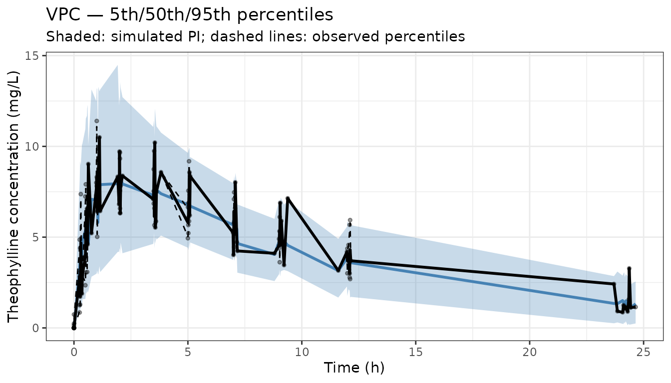
Stratified VPC
For covariate-stratified VPCs, split both observed and simulated data
by the covariate before computing percentiles, then use
facet_wrap():
# Create a weight group (above/below median)
medWt <- median(obs$WT)
obs$wtGrp    <- ifelse(obs$WT >= medWt, "WT >= median", "WT < median")
simDat$wtGrp <- ifelse(simDat$WT >= medWt, "WT >= median", "WT < median")

simDT2  <- as.data.table(simDat)
obsDT2  <- as.data.table(obs[obs$EVID == 0, ])

simPctl2 <- simDT2[, .(
  p05 = quantile(sim, 0.05, na.rm = TRUE),
  p50 = quantile(sim, 0.50, na.rm = TRUE),
  p95 = quantile(sim, 0.95, na.rm = TRUE)
), by = .(time, wtGrp)]
setnames(simPctl2, "time", "TIME")

obsPctl2 <- obsDT2[, .(
  p05 = quantile(DV, 0.05, na.rm = TRUE),
  p50 = quantile(DV, 0.50, na.rm = TRUE),
  p95 = quantile(DV, 0.95, na.rm = TRUE)
), by = .(TIME, wtGrp)]

ggplot() +
  geom_ribbon(data = simPctl2,
              aes(x = TIME, ymin = p05, ymax = p95),
              fill = "steelblue", alpha = 0.3) +
  geom_line(data = simPctl2,
            aes(x = TIME, y = p50),
            colour = "steelblue", linewidth = 1) +
  geom_line(data = obsPctl2,
            aes(x = TIME, y = p50),
            colour = "black", linewidth = 1) +
  geom_point(data = obsDT2,
             aes(x = TIME, y = DV),
             alpha = 0.3, size = 1) +
  facet_wrap(~wtGrp) +
  labs(x = "Time (h)", y = "Concentration (mg/L)",
       title = "Stratified VPC by weight group") +
  theme_bw()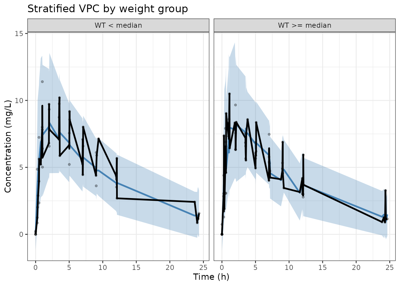
Tips
- Use at least 500 replicates for stable 5th/95th percentile estimates.
- For log-scale PK data add
scale_y_log10()to the ggplot. - For censored data (
CENS=1) usevpc_cens()from thevpcpackage. - For time-to-event models use
vpc_tte(). - Binning strategy (equal-width, equal-count, or user-defined)
strongly affects VPC appearance; the
vpcpackage provides several options via thebinsargument.