Introduction to rxode2

Introduction

rxode2 is an R package that facilitates simulation with ODE models in R. It is designed with pharmacometrics models in mind, but can be applied more generally to any ODE model.

Description of rxode2 illustrated through an example

The model equations can be specified through a text string, a model file or an R expression. Both differential and algebraic equations are permitted. Differential equations are specified by d/dt(var_name) =. Each equation can be separated by a semicolon.

To load rxode2 package and compile the model:

library(rxode2)
#> rxode2 2.1.2.9000 using 2 threads (see ?getRxThreads)
#>   no cache: create with `rxCreateCache()`

mod1 <- function() {
  ini({
    # central 
    KA=2.94E-01
    CL=1.86E+01
    V2=4.02E+01
    # peripheral
    Q=1.05E+01
    V3=2.97E+02
    # effects
    Kin=1
    Kout=1
    EC50=200 
  })
  model({
    C2 <- centr/V2
    C3 <- peri/V3
    d/dt(depot) <- -KA*depot
    d/dt(centr) <- KA*depot - CL*C2 - Q*C2 + Q*C3
    d/dt(peri)  <- Q*C2 - Q*C3
    eff(0) <- 1
    d/dt(eff)   <- Kin - Kout*(1-C2/(EC50+C2))*eff
  })
}

Model parameters may be specified in the ini({}) model block, initial conditions can be specified within the model with the cmt(0)= X, like in this model eff(0) <- 1.

You may also specify between subject variability initial conditions and residual error components just like nlmixr2. This allows a single interface for nlmixr2/rxode2 models. Also note, the classic rxode2 interface still works just like it did in the past (so don’t worry about breaking code at this time).

In fact, you can get the classic rxode2 model $simulationModel in the ui object:

mod1 <- mod1() # create the ui object (can also use `rxode2(mod1)`)
mod1

summary(mod1$simulationModel)

Specify Dosing and sampling in rxode2

rxode2 provides a simple and very flexible way to specify dosing and sampling through functions that generate an event table. First, an empty event table is generated through the “et()” function. This has an interface that is similar to NONMEM event tables:

ev  <- et(amountUnits="mg", timeUnits="hours") %>%
  et(amt=10000, addl=9,ii=12,cmt="depot") %>%
  et(time=120, amt=2000, addl=4, ii=14, cmt="depot") %>%
  et(0:240) # Add sampling

You can see from the above code, you can dose to the compartment named in the rxode2 model. This slight deviation from NONMEM can reduce the need for compartment renumbering.

These events can also be combined and expanded (to multi-subject events and complex regimens) with rbind, c, seq, and rep. For more information about creating complex dosing regimens using rxode2 see the rxode2 events vignette.

Solving ODEs

The ODE can now be solved using rxSolve:

x <- mod1 %>% rxSolve(ev)
#> using C compiler: ‘gcc (Ubuntu 11.4.0-1ubuntu1~22.04) 11.4.0’
x
#> ── Solved rxode2 object ──
#> ── Parameters (x$params): ──
#>      KA      CL      V2       Q      V3     Kin    Kout    EC50 
#>   0.294  18.600  40.200  10.500 297.000   1.000   1.000 200.000 
#> ── Initial Conditions (x$inits): ──
#> depot centr  peri   eff 
#>     0     0     0     1 
#> ── First part of data (object): ──
#> # A tibble: 241 × 7
#>   time    C2    C3  depot centr  peri   eff
#>    [h] <dbl> <dbl>  <dbl> <dbl> <dbl> <dbl>
#> 1    0   0   0     10000     0     0   1   
#> 2    1  44.4 0.920  7453. 1784.  273.  1.08
#> 3    2  54.9 2.67   5554. 2206.  794.  1.18
#> 4    3  51.9 4.46   4140. 2087. 1324.  1.23
#> 5    4  44.5 5.98   3085. 1789. 1776.  1.23
#> 6    5  36.5 7.18   2299. 1467. 2132.  1.21
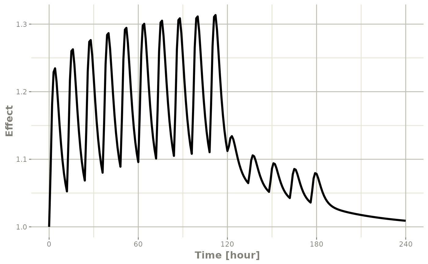
#> # ℹ 235 more rows

This returns a modified data frame. You can see the compartment values in the plot below:

library(ggplot2)
plot(x,C2) + ylab("Central Concentration")

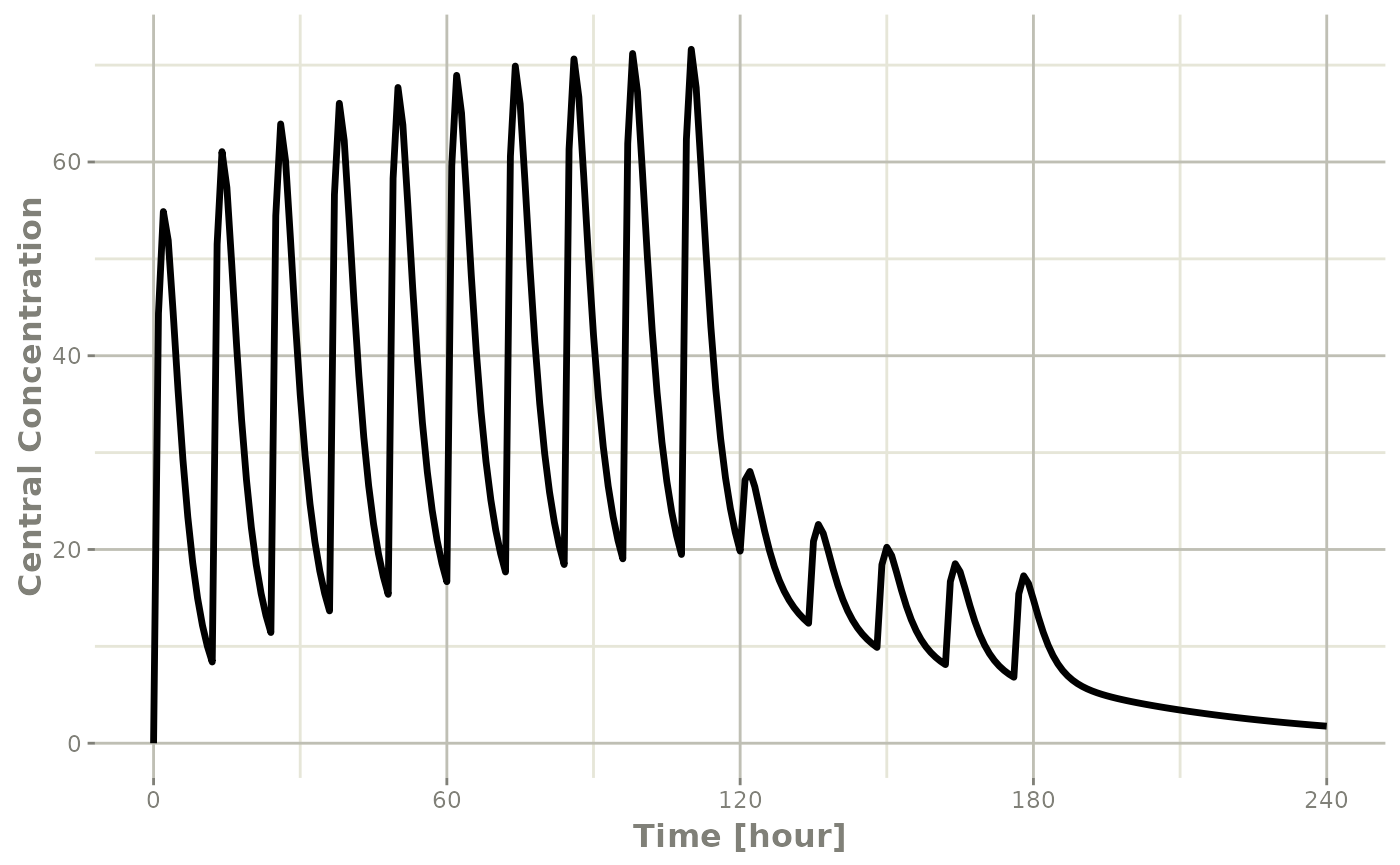
Or,

plot(x,eff)  + ylab("Effect")

Note that the labels are automatically labeled with the units from the initial event table. rxode2 extracts units to label the plot (if they are present).

2024-04-16

Introduction

Description of rxode2 illustrated through an example

Specify Dosing and sampling in rxode2

Solving ODEs