Individual Covariates
If there is an individual covariate you wish to solve for you may
specify it by the iCov dataset:
## rxode2 5.1.5 using 2 threads (see ?getRxThreads)
## no cache: create with `rxCreateCache()`## udunits database from /usr/share/xml/udunits/udunits2.xml
library(xgxr)

mod3 <- function() {
  ini({
    TKA   <- 2.94E-01
    ## Clearance with individuals
    TCL   <- 1.86E+01
    TV2   <-4.02E+01
    TQ    <-1.05E+01
    TV3   <-2.97E+02
    TKin  <- 1
    TKout <- 1
    TEC50 <-200
  })
  model({
    KA            <- TKA
    CL            <- TCL * (WT / 70) ^ 0.75
    V2            <- TV2
    Q             <- TQ
    V3            <- TV3
    Kin           <- TKin
    Kout          <- TKout
    EC50          <- TEC50
    Tz            <- 8
    amp           <- 0.1
    C2            <- central/V2
    C3            <- peri/V3
    d/dt(depot)   <- -KA*depot
    d/dt(central) <- KA*depot - CL*C2 - Q*C2 + Q*C3
    d/dt(peri)    <-                    Q*C2 - Q*C3
    d/dt(eff)     <-  Kin - Kout*(1-C2/(EC50+C2))*eff
    eff(0)        <- 1  ## This specifies that the effect compartment starts at 1.
  })
}

ev <- et(amount.units="mg", time.units="hours") |>
  et(amt=10000, cmt=1) |>
  et(0,48,length.out=100) |>
  et(id=1:4)

set.seed(10)
rxSetSeed(10)
## Now use iCov to simulate a 4-id sample
r1 <- solve(mod3, ev,
            # Create individual covariate data-frame
            iCov=data.frame(id=1:4, WT=rnorm(4, 70, 10)))
## ℹ parameter labels from comments are typically ignored in non-interactive mode## ℹ Need to run with the source intact to parse comments
print(r1)## ── Solved rxode2 object ──
## ── Parameters ($params): ──
## TKA TCL TV2 TQ TV3 TKin TKout TEC50 Tz amp
## 0.294 18.600 40.200 10.500 297.000 1.000 1.000 200.000 8.000 0.100
## ── Initial Conditions ($inits): ──
## depot central peri eff
## 0 0 0 1
## ── First part of data (object): ──
## # A tibble: 400 × 17
## id time KA CL V2 Q V3 Kin Kout EC50 C2 C3 depot
## <int> [h] <dbl> <dbl> <dbl> <dbl> <dbl> <dbl> <dbl> <dbl> <dbl> <dbl> <dbl>
## 1 3 0 0.294 15.8 40.2 10.5 297 1 1 200 0 0 10000
## 2 3 0.485 0.294 15.8 40.2 10.5 297 1 1 200 28.2 0.260 8671.
## 3 3 0.970 0.294 15.8 40.2 10.5 297 1 1 200 45.1 0.892 7519.
## 4 3 1.45 0.294 15.8 40.2 10.5 297 1 1 200 54.2 1.73 6520.
## 5 3 1.94 0.294 15.8 40.2 10.5 297 1 1 200 58.1 2.66 5654.
## 6 3 2.42 0.294 15.8 40.2 10.5 297 1 1 200 58.6 3.61 4903.
## # ℹ 394 more rows
## # ℹ 4 more variables: central <dbl>, peri <dbl>, eff <dbl>, WT <dbl>
plot(r1, C2, log="y")## Warning in ggplot2::scale_y_log10(..., breaks = breaks, minor_breaks =
## minor_breaks, : log-10 transformation introduced infinite
## values.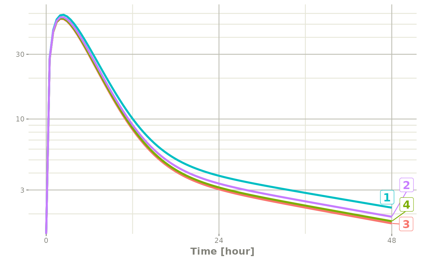
Time Varying Covariates
Covariates are easy to specify in rxode2, you can specify them as a variable. Time-varying covariates, like clock time in a circadian rhythm model, can also be used. Extending the indirect response model already discussed, we have:
library(rxode2)
library(units)

mod4 <- mod3 |>
  model(d/dt(eff) <-  Kin - Kout*(1-C2/(EC50+C2))*eff) |>
  model(-Kin) |>
  model(Kin <- TKin + amp *cos(2*pi*(ctime-Tz)/24), append=C2, cov="ctime")

ev <- et(amountUnits="mg", timeUnits="hours") |>
    et(amt=10000, cmt=1) |>
    et(0,48,length.out=100)


## Create data frame of 8 am dosing for the first dose This is done
## with base R but it can be done with dplyr or data.table
ev$ctime <- (ev$time+set_units(8,hr)) %% 24
ev$WT <- 70
Now there is a covariate present in the event dataset, the system can be solved by combining the dataset and the model:
r1 <- solve(mod4, ev, covsInterpolation="linear")
print(r1)
#> ── Solved rxode2 object ──
#> ── Parameters ($params): ──
#>        TKA        TCL        TV2         TQ        TV3      TKout      TEC50
#>   0.294000  18.600000  40.200000  10.500000 297.000000   1.000000 200.000000
#>       TKin         Tz        amp         pi
#>   1.000000   8.000000   0.100000   3.141593
#> ── Initial Conditions ($inits): ──
#>   depot central    peri     eff
#>       0       0       0       1
#> ── First part of data (object): ──
#> # A tibble: 100 × 17
#>    time    KA    CL    V2     Q    V3  Kout  EC50    C2   Kin    C3  depot
#>     [h] <dbl> <dbl> <dbl> <dbl> <dbl> <dbl> <dbl> <dbl> <dbl> <dbl>  <dbl>
#> 1 0     0.294  18.6  40.2  10.5   297     1   200   0    1.1  0     10000
#> 2 0.485 0.294  18.6  40.2  10.5   297     1   200  27.8  1.10 0.257  8671.
#> 3 0.970 0.294  18.6  40.2  10.5   297     1   200  43.7  1.10 0.874  7519.
#> 4 1.45  0.294  18.6  40.2  10.5   297     1   200  51.8  1.09 1.68   6520.
#> 5 1.94  0.294  18.6  40.2  10.5   297     1   200  54.8  1.09 2.56   5654.
#> 6 2.42  0.294  18.6  40.2  10.5   297     1   200  54.6  1.08 3.45   4903.
#> # ℹ 94 more rows
#> # ℹ 5 more variables: central <dbl>, peri <dbl>, eff <dbl>, ctime <dbl>,
#> #   WT <dbl>
When solving ODE equations, the solver may sample times outside of
the data. When this happens, this ODE solver can use linear
interpolation between the covariate values. It is equivalent to R’s
approxfun with method="linear".
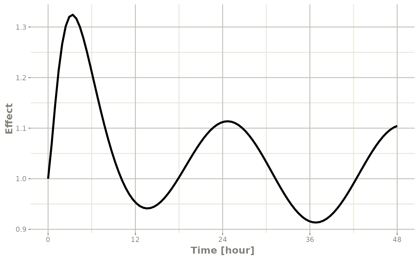
plot(r1,C2, ylab="Central Concentration")
Note that the linear approximation in this case leads to some kinks in the solved system at 24-hours where the covariate has a linear interpolation between near 24 and near 0. While linear seems reasonable, cases like clock time make other interpolation methods more attractive.
In rxode2 the default covariate interpolation is be the last
observation carried forward (locf), or constant
approximation. This is equivalent to R’s approxfun with
method="constant".
r1 <- solve(mod4, ev,covsInterpolation="locf")
print(r1)
#> ── Solved rxode2 object ──
#> ── Parameters ($params): ──
#>        TKA        TCL        TV2         TQ        TV3      TKout      TEC50
#>   0.294000  18.600000  40.200000  10.500000 297.000000   1.000000 200.000000
#>       TKin         Tz        amp         pi
#>   1.000000   8.000000   0.100000   3.141593
#> ── Initial Conditions ($inits): ──
#>   depot central    peri     eff
#>       0       0       0       1
#> ── First part of data (object): ──
#> # A tibble: 100 × 17
#>    time    KA    CL    V2     Q    V3  Kout  EC50    C2   Kin    C3  depot
#>     [h] <dbl> <dbl> <dbl> <dbl> <dbl> <dbl> <dbl> <dbl> <dbl> <dbl>  <dbl>
#> 1 0     0.294  18.6  40.2  10.5   297     1   200   0    1.1  0     10000
#> 2 0.485 0.294  18.6  40.2  10.5   297     1   200  27.8  1.10 0.257  8671.
#> 3 0.970 0.294  18.6  40.2  10.5   297     1   200  43.7  1.10 0.874  7519.
#> 4 1.45  0.294  18.6  40.2  10.5   297     1   200  51.8  1.09 1.68   6520.
#> 5 1.94  0.294  18.6  40.2  10.5   297     1   200  54.8  1.09 2.56   5654.
#> 6 2.42  0.294  18.6  40.2  10.5   297     1   200  54.6  1.08 3.45   4903.
#> # ℹ 94 more rows
#> # ℹ 5 more variables: central <dbl>, peri <dbl>, eff <dbl>, ctime <dbl>,
#> #   WT <dbl>
which gives the following plots:
plot(r1,C2, ylab="Central Concentration", xlab="Time")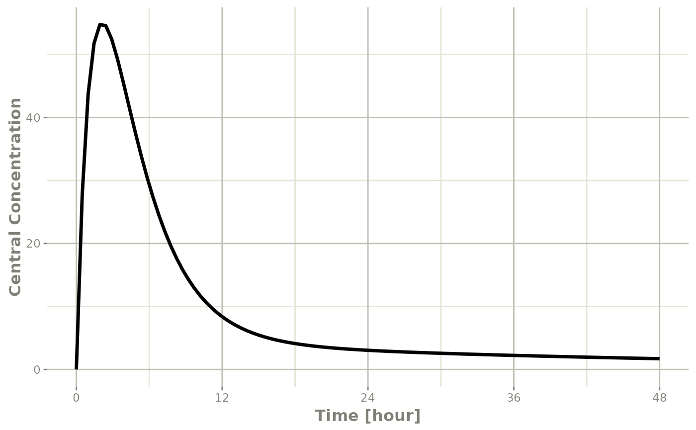
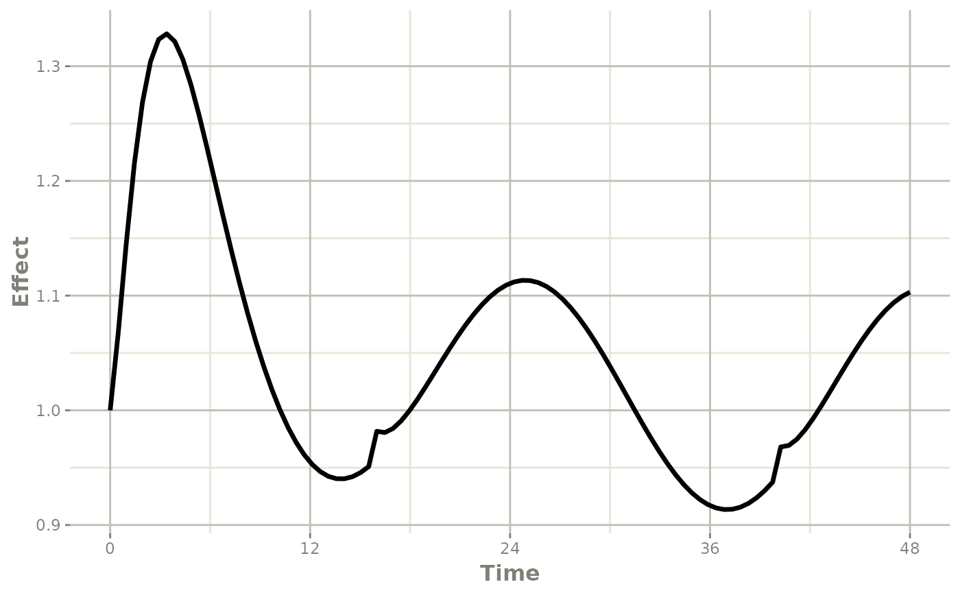
plot(r1,eff, ylab="Effect", xlab="Time")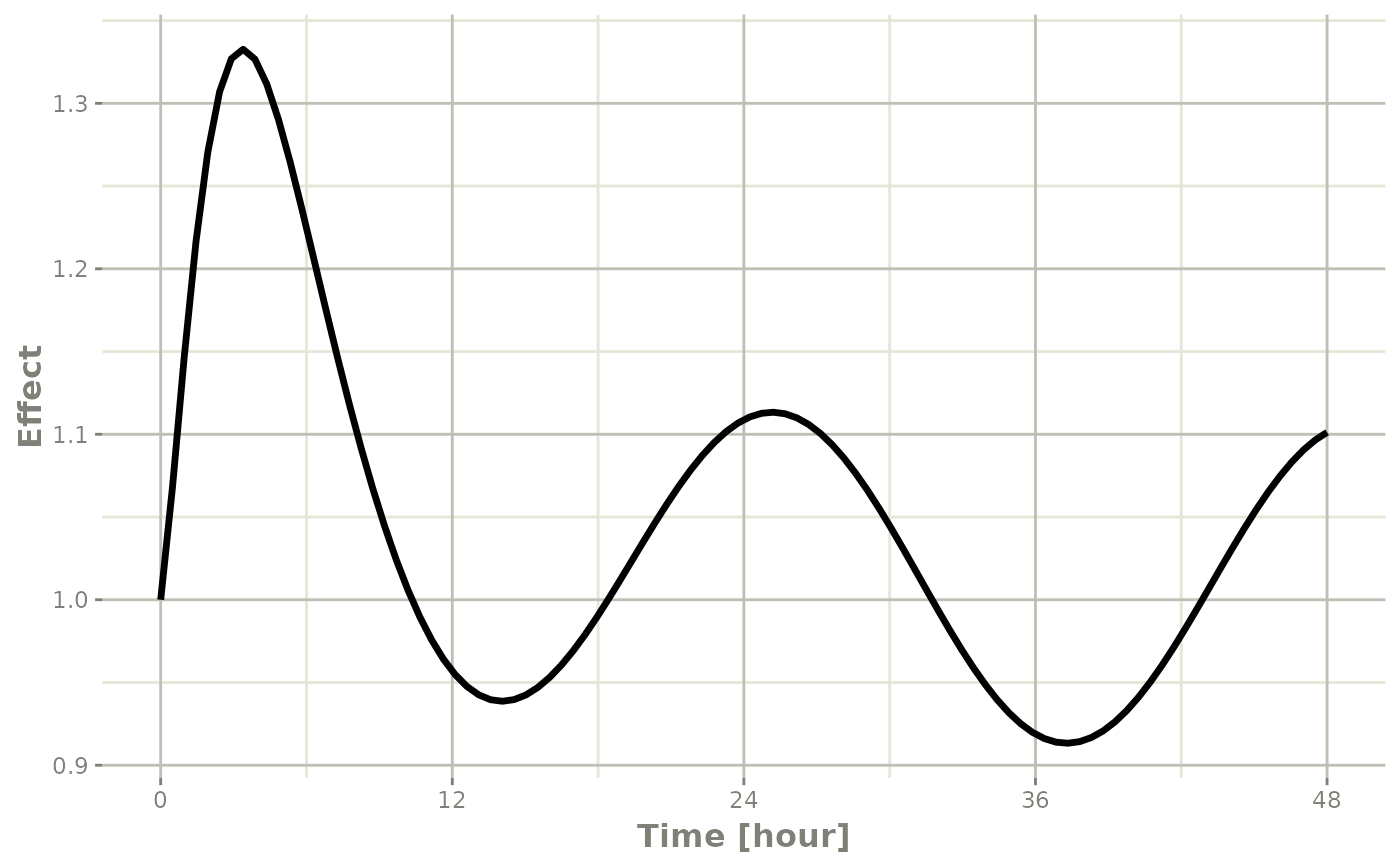
In this case, the plots seem to be smoother.
You can also use NONMEM’s preferred interpolation style of next observation carried backward (NOCB):
r1 <- solve(mod4, ev,covsInterpolation="nocb")
print(r1)
#> ── Solved rxode2 object ──
#> ── Parameters ($params): ──
#>        TKA        TCL        TV2         TQ        TV3      TKout      TEC50
#>   0.294000  18.600000  40.200000  10.500000 297.000000   1.000000 200.000000
#>       TKin         Tz        amp         pi
#>   1.000000   8.000000   0.100000   3.141593
#> ── Initial Conditions ($inits): ──
#>   depot central    peri     eff
#>       0       0       0       1
#> ── First part of data (object): ──
#> # A tibble: 100 × 17
#>    time    KA    CL    V2     Q    V3  Kout  EC50    C2   Kin    C3  depot
#>     [h] <dbl> <dbl> <dbl> <dbl> <dbl> <dbl> <dbl> <dbl> <dbl> <dbl>  <dbl>
#> 1 0     0.294  18.6  40.2  10.5   297     1   200   0    1.1  0     10000
#> 2 0.485 0.294  18.6  40.2  10.5   297     1   200  27.8  1.10 0.257  8671.
#> 3 0.970 0.294  18.6  40.2  10.5   297     1   200  43.7  1.10 0.874  7519.
#> 4 1.45  0.294  18.6  40.2  10.5   297     1   200  51.8  1.09 1.68   6520.
#> 5 1.94  0.294  18.6  40.2  10.5   297     1   200  54.8  1.09 2.56   5654.
#> 6 2.42  0.294  18.6  40.2  10.5   297     1   200  54.6  1.08 3.45   4903.
#> # ℹ 94 more rows
#> # ℹ 5 more variables: central <dbl>, peri <dbl>, eff <dbl>, ctime <dbl>,
#> #   WT <dbl>
which gives the following plots:
plot(r1,C2, ylab="Central Concentration", xlab="Time")
plot(r1,eff, ylab="Effect", xlab="Time")