rxode2 Datasets and Event Types

rxode2 event tables

In general, rxode2 event tables follow NONMEM dataset conventions with the following exceptions and extensions:

The compartment data item (cmt) can be a string/factor with compartment names.
- You may turn off a compartment with a negative compartment number or "-cmt" where cmt is the compartment name.
- The compartment data item (cmt) can still be a number; the number of a compartment is defined by the order of appearance of its name in the model. You can assign compartment numbers explicitly with cmt(cmtName) at the beginning of the model.
An additional column dur can specify the duration of infusions:
- Bioavailability changes will change the rate of infusion when dur/amt are fixed in the input data.
- Similarly, when specifying rate/amt for an infusion, bioavailability changes will alter the infusion duration since rate/amt are fixed.
Some infrequent NONMEM columns are not supported: pcmt, call.
NONMEM-style events are supported (0: Observation, 1: Dose, 2: Other, 3: Reset, 4: Reset+Dose). Additional events are supported:
- evid=5 or replace event: replaces the value of a compartment with the value specified in the amt column (equivalent to deSolve replace).
- evid=6 or multiply event: multiplies the compartment value by the amt column (equivalent to deSolve multiply).
- evid=7 or transit/phantom event: puts the dose in the dose() function and calculates time since last dose tad(), but does not place the dose in the compartment. This allows the transit() function to be applied easily.

Dataset column reference

Columns by type of use

Data for input into rxode2 (and nlmixr2) is similar to NONMEM data; most NONMEM-ready datasets can be used directly.

Subject identification

Column	Meaning
`ID`	Subject identifier — integer, character, or factor

Observation columns

Column	Meaning
`DV`	Dependent variable (measurement)
`CENS`	Censoring indicator (0 = not censored, 1 = left censored, -1 = right censored)
`LIMIT`	Censoring bound used with `CENS` (see below)
`MDV`	Missing dependent variable indicator
`CMT`	Compartment name or number for the observation
`DVID`	Dependent variable identifier for multiple endpoints
`EVID`	Event identifier

Dosing columns

Column	Meaning
`AMT`	Dose amount
`CMT`	Compartment name or number for the dose
`EVID`	Event identifier
`ADDL`	Number of additional doses identical to this one
`II`	Inter-dose interval
`RATE` or `DUR`	Infusion rate or duration
`SS`	Steady-state flag

Complete column quick-reference table

Data Item	Meaning	Notes
`id`	Individual identifier	Integer, factor, character, or numeric
`time`	Individual time	Numeric
`amt`	Dose amount	Positive for doses; zero/NA for observations
`rate`	Infusion rate	Duration = `amt/rate`; `rate=-1`: rate modeled; `rate=-2`: duration modeled
`dur`	Infusion duration	Rate = `amt/dur`
`evid`	Event ID	0=Obs; 1=Dose; 2=Other; 3=Reset; 4=Reset+Dose; 5=Replace; 6=Multiply; 7=Transit
`cmt`	Compartment	Name or number; prefix `-` to turn off
`ss`	Steady-state flag	0=non-SS; 1=SS; 2=SS + keep prior states
`ii`	Inter-dose interval	Time between doses
`addl`	Additional doses	Number of doses identical to this one
`dvid`	DV identifier	Identifies which endpoint an observation belongs to

Per-column details

`AMT` column

The AMT column defines the amount of a dose administered to CMT. For observation rows it should be 0 or NA. For zero-order infusions the rate or duration is set via RATE or DUR.

`CENS` / `LIMIT` columns

CENS indicates whether the observation in DV is censored:

CENS = 0: not censored; LIMIT is ignored.
CENS = 1: left censored (e.g., below the limit of quantification); the true value lies in (LIMIT, DV).
CENS = -1: right censored (above limit of quantification); the true value lies in (DV, LIMIT).

rxode2 stores these values so that nlmixr2 can use them in likelihood calculations.

`CMT` column

CMT indicates the compartment where an event occurs. A character string or factor (the preferred form) is matched by name in the model. An integer is matched by the order in which compartments appear in the model. Prefix with - (e.g. cmt="-depot") to turn off a compartment.

`DUR` column

DUR defines the duration of a zero-order infusion. When DUR is specified, the infusion rate is computed as rate = amt/dur. Bioavailability changes affect the rate, not the duration.

`DV` column

DV is the dependent variable in the observation compartment defined by CMT / DVID. It may be missing (MDV=1) or censored (CENS≠0).

`DVID` column

DVID identifies which endpoint an observation belongs to in multi-endpoint models. It maps to the cond field in $predDf and can be specified as a name (matching the endpoint variable) or integer.

`EVID` column

The event identifier for a row of data:

`EVID`	Meaning
0	Observation
1	Dose
2	Other (e.g. turn off compartment)
3	Reset all compartments to initial values
4	Reset + dose
5	Replace compartment value with `amt`
6	Multiply compartment value by `amt`
7	Transit/phantom dose (`dose()` / `tad()` only)

Output-only EVID values (visible when addDosing=TRUE, subsetNonmem=FALSE):

`EVID`	Meaning
-1	Modeled-rate infusion end (`rate=-1`)
-2	Modeled-duration infusion end (`rate=-2`)
-10	Rate-specified infusion end (`rate>0`)
-20	Duration-specified infusion end (`dur>0`)
101, 102, …	Modeled times 1, 2, … (`mtime`)

Use addDosing=NA to see classic EVID equivalents instead.

`ID` column

ID separates individuals (persons, animals, etc.). The solver re-initialises the numerical integrator and samples new random effects with each new ID. It may be an integer, character, or factor.

`RATE` column

RATE specifies a zero-order infusion rate. The infusion duration is computed as dur = amt/rate. Special values:

rate = -1: rate is modeled (set via rate(cmt) in the model block); equivalent to NONMEM RATE=-1.
rate = -2: duration is modeled (set via dur(cmt) in the model block); equivalent to NONMEM RATE=-2.

When RATE is fixed in the dataset, a bioavailability change alters the infusion duration. When DUR is fixed instead, a bioavailability change alters the infusion rate.

Other notes:

NONMEM’s DV is not required; rxode2 is an ODE solving framework and DV is only used by nlmixr2.
NONMEM’s MDV is not required; missingness is captured in EVID.
Instead of NONMEM-compatible data, deSolve-compatible data frames are also accepted.
The classic RxODE EVID encoding is also supported (see Classic rxode2 Events).

Event type examples

To illustrate each event type, the following model from the original rxode2 tutorial is used throughout:

library(rxode2)

#> rxode2 5.0.2 using 2 threads (see ?getRxThreads)
#>   no cache: create with `rxCreateCache()`

m1 <- function() {
  ini({
    KA   <- 2.94E-01
    CL   <- 1.86E+01
    V2   <- 4.02E+01
    Q    <- 1.05E+01
    V3   <- 2.97E+02
    Kin  <- 1
    Kout <- 1
    EC50 <- 200
    ## Modeled bioavailability, duration and rate
    fdepot    <- 1
    durDepot  <- 8
    rateDepot <- 1250
  })
  model({
    C2 <- centr/V2
    C3 <- peri/V3
    d/dt(depot) <- -KA*depot
    f(depot)    <- fdepot
    dur(depot)  <- durDepot
    rate(depot) <- rateDepot
    d/dt(centr) <- KA*depot - CL*C2 - Q*C2 + Q*C3
    d/dt(peri)  <-                    Q*C2 - Q*C3
    d/dt(eff)   <- Kin - Kout*(1-C2/(EC50+C2))*eff
    eff(0) <- 1
  })
}

Bolus/Additive Doses

A bolus dose is the default dose type and only requires amt.

ev <- et(timeUnits="hr") |>
    et(amt=10000, ii=12, until=24) |>
    et(seq(0, 24, length.out=100))

ev

#> -- EventTable with 101 records --
#> 1 dosing records (see x$get.dosing(); add with add.dosing or et)
#> 100 observation times (see x$get.sampling(); add with add.sampling or et)
#> multiple doses in `addl` columns, expand with x$expand(); or etExpand(x)
#> -- First part of x: --
#> # A tibble: 101 x 5
#>     time   amt  ii  addl evid         
#>      [h] <dbl> [h] <int> <evid>       
#>  1 0        NA  NA    NA 0:Observation
#>  2 0     10000  12     2 1:Dose (Add) 
#>  3 0.242    NA  NA    NA 0:Observation
#>  4 0.485    NA  NA    NA 0:Observation
#>  5 0.727    NA  NA    NA 0:Observation
#>  6 0.970    NA  NA    NA 0:Observation
#>  7 1.21     NA  NA    NA 0:Observation
#>  8 1.45     NA  NA    NA 0:Observation
#>  9 1.70     NA  NA    NA 0:Observation
#> 10 1.94     NA  NA    NA 0:Observation
#> # i 91 more rows

rxSolve(m1, ev) |> plot(C2) +
    xlab("Time")

#> i parameter labels from comments are typically ignored in non-interactive mode

#> i Need to run with the source intact to parse comments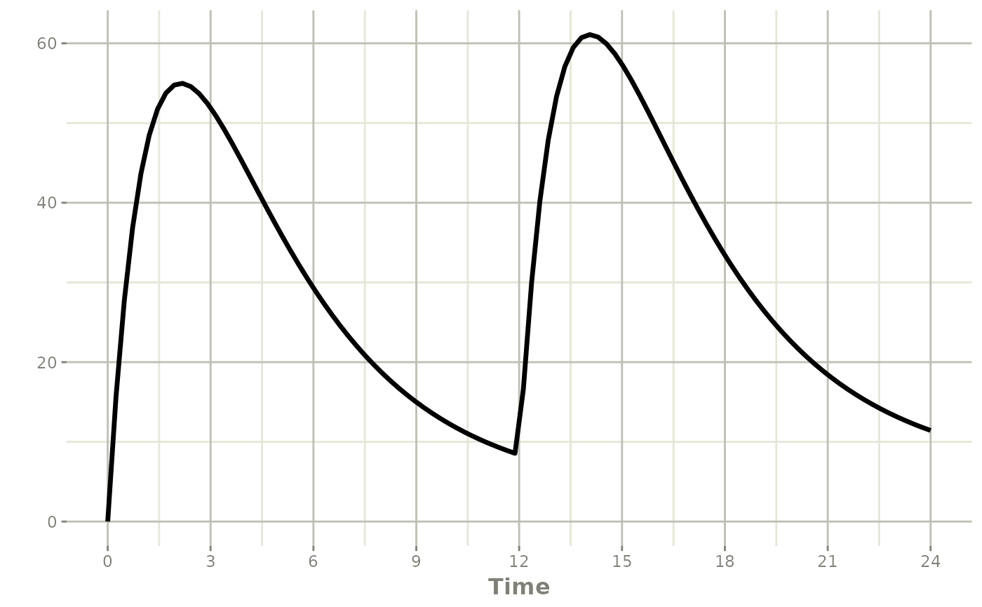

Infusion Doses

rxode2 supports several infusion types:

Constant rate infusion (rate)
Constant duration infusion (dur)
Estimated (modeled) rate of infusion
Estimated (modeled) duration of infusion

Constant infusion specified by duration or rate

Using `dur`

ev <- et(timeUnits="hr") |>
    et(amt=10000, ii=12, until=24, dur=8) |>
    et(seq(0, 24, length.out=100))

ev

#> -- EventTable with 101 records --
#> 1 dosing records (see x$get.dosing(); add with add.dosing or et)
#> 100 observation times (see x$get.sampling(); add with add.sampling or et)
#> multiple doses in `addl` columns, expand with x$expand(); or etExpand(x)
#> -- First part of x: --
#> # A tibble: 101 x 6
#>     time   amt  ii  addl evid          dur
#>      [h] <dbl> [h] <int> <evid>        [h]
#>  1 0        NA  NA    NA 0:Observation  NA
#>  2 0     10000  12     2 1:Dose (Add)    8
#>  3 0.242    NA  NA    NA 0:Observation  NA
#>  4 0.485    NA  NA    NA 0:Observation  NA
#>  5 0.727    NA  NA    NA 0:Observation  NA
#>  6 0.970    NA  NA    NA 0:Observation  NA
#>  7 1.21     NA  NA    NA 0:Observation  NA
#>  8 1.45     NA  NA    NA 0:Observation  NA
#>  9 1.70     NA  NA    NA 0:Observation  NA
#> 10 1.94     NA  NA    NA 0:Observation  NA
#> # i 91 more rows

rxSolve(m1, ev) |> plot(depot, C2) +
    xlab("Time")

#> i parameter labels from comments are typically ignored in non-interactive mode

#> i Need to run with the source intact to parse comments

Using `rate`

ev <- et(timeUnits="hr") |>
    et(amt=10000, ii=12, until=24, rate=10000/8) |>
    et(seq(0, 24, length.out=100))

ev

#> -- EventTable with 101 records --
#> 1 dosing records (see x$get.dosing(); add with add.dosing or et)
#> 100 observation times (see x$get.sampling(); add with add.sampling or et)
#> multiple doses in `addl` columns, expand with x$expand(); or etExpand(x)
#> -- First part of x: --
#> # A tibble: 101 x 6
#>     time   amt rate        ii  addl evid         
#>      [h] <dbl> <rate/dur> [h] <int> <evid>       
#>  1 0        NA NA          NA    NA 0:Observation
#>  2 0     10000  1250       12     2 1:Dose (Add) 
#>  3 0.242    NA NA          NA    NA 0:Observation
#>  4 0.485    NA NA          NA    NA 0:Observation
#>  5 0.727    NA NA          NA    NA 0:Observation
#>  6 0.970    NA NA          NA    NA 0:Observation
#>  7 1.21     NA NA          NA    NA 0:Observation
#>  8 1.45     NA NA          NA    NA 0:Observation
#>  9 1.70     NA NA          NA    NA 0:Observation
#> 10 1.94     NA NA          NA    NA 0:Observation
#> # i 91 more rows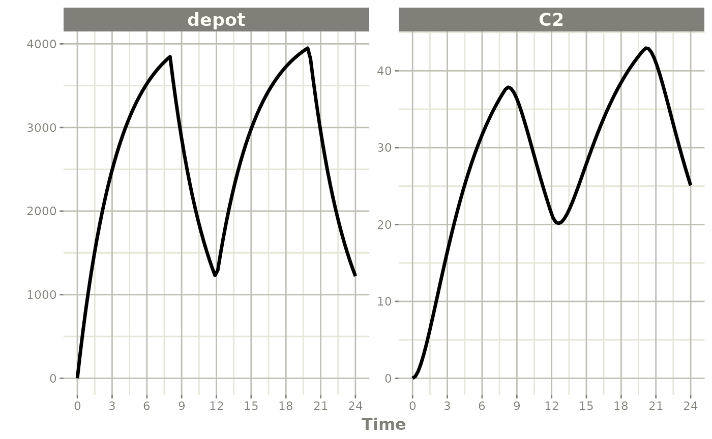

rxSolve(m1, ev) |> plot(depot, C2) +
    xlab("Time")

#> i parameter labels from comments are typically ignored in non-interactive mode

#> i Need to run with the source intact to parse comments

The two specifications produce the same nominal infusion. The difference appears when bioavailability changes.

When rate is fixed in the event table, a bioavailability decrease shortens the infusion duration (as in NONMEM):

rxSolve(m1, ev, c(fdepot=0.25)) |> plot(depot, C2) + xlab("Time")

#> i parameter labels from comments are typically ignored in non-interactive mode

#> i Need to run with the source intact to parse comments

rxSolve(m1, ev, c(fdepot=1.25)) |> plot(depot, C2) + xlab("Time")

#> i parameter labels from comments are typically ignored in non-interactive mode
#> i Need to run with the source intact to parse comments

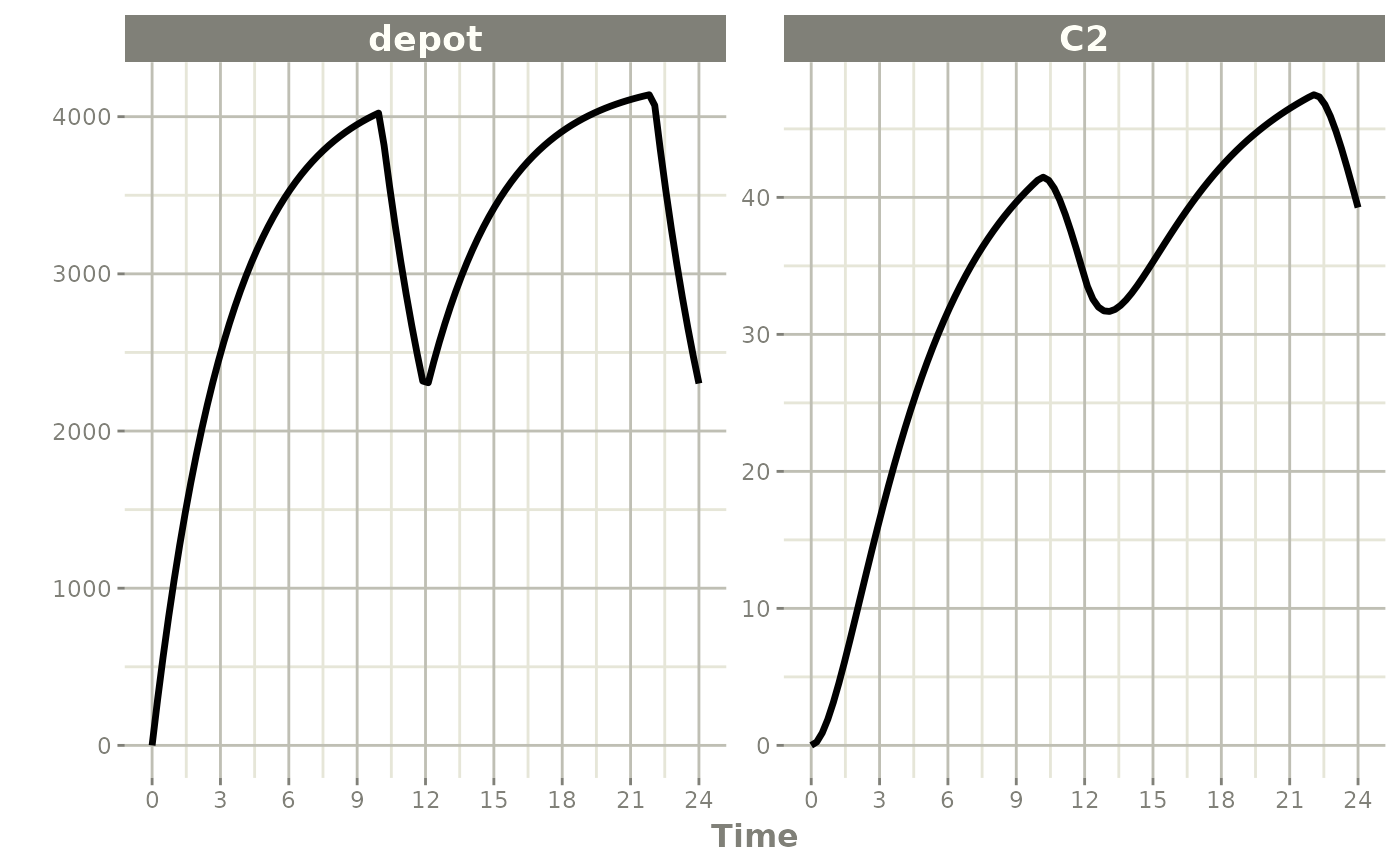
When dur is fixed instead, a bioavailability change alters the infusion rate:

ev <- et(timeUnits="hr") |>
    et(amt=10000, ii=12, until=24, dur=8) |>
    et(seq(0, 24, length.out=100))

library(ggplot2)
library(patchwork)

p1 <- rxSolve(m1, ev, c(fdepot=1.25)) |> plot(depot) +
    xlab("Time") + ylim(0, 5000)

#> i parameter labels from comments are typically ignored in non-interactive mode

#> i Need to run with the source intact to parse comments

p2 <- rxSolve(m1, ev, c(fdepot=0.25)) |> plot(depot) +
    xlab("Time") + ylim(0, 5000)

#> i parameter labels from comments are typically ignored in non-interactive mode
#> i Need to run with the source intact to parse comments

p1 * p2

Modeled rate and duration of infusion

Model the infusion duration (rate=-2, equivalent to NONMEM RATE=-2):

ev <- et(timeUnits="hr") |>
    et(amt=10000, ii=12, until=24, rate=-2) |>
    et(seq(0, 24, length.out=100))

ev

#> -- EventTable with 101 records --
#> 1 dosing records (see x$get.dosing(); add with add.dosing or et)
#> 100 observation times (see x$get.sampling(); add with add.sampling or et)
#> multiple doses in `addl` columns, expand with x$expand(); or etExpand(x)
#> -- First part of x: --
#> # A tibble: 101 x 6
#>     time   amt rate        ii  addl evid         
#>      [h] <dbl> <rate/dur> [h] <int> <evid>       
#>  1 0        NA NA          NA    NA 0:Observation
#>  2 0     10000 -2:dur      12     2 1:Dose (Add) 
#>  3 0.242    NA NA          NA    NA 0:Observation
#>  4 0.485    NA NA          NA    NA 0:Observation
#>  5 0.727    NA NA          NA    NA 0:Observation
#>  6 0.970    NA NA          NA    NA 0:Observation
#>  7 1.21     NA NA          NA    NA 0:Observation
#>  8 1.45     NA NA          NA    NA 0:Observation
#>  9 1.70     NA NA          NA    NA 0:Observation
#> 10 1.94     NA NA          NA    NA 0:Observation
#> # i 91 more rows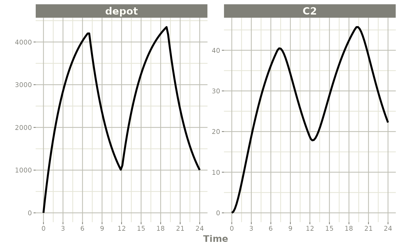

rxSolve(m1, ev, c(durDepot=7)) |> plot(depot, C2) + xlab("Time")

#> i parameter labels from comments are typically ignored in non-interactive mode

#> i Need to run with the source intact to parse comments

Model the infusion rate (rate=-1, equivalent to NONMEM RATE=-1):

ev <- et(timeUnits="hr") |>
    et(amt=10000, ii=12, until=24, rate=-1) |>
    et(seq(0, 24, length.out=100))

ev

#> -- EventTable with 101 records --
#> 1 dosing records (see x$get.dosing(); add with add.dosing or et)
#> 100 observation times (see x$get.sampling(); add with add.sampling or et)
#> multiple doses in `addl` columns, expand with x$expand(); or etExpand(x)
#> -- First part of x: --
#> # A tibble: 101 x 6
#>     time   amt rate        ii  addl evid         
#>      [h] <dbl> <rate/dur> [h] <int> <evid>       
#>  1 0        NA NA          NA    NA 0:Observation
#>  2 0     10000 -1:rate     12     2 1:Dose (Add) 
#>  3 0.242    NA NA          NA    NA 0:Observation
#>  4 0.485    NA NA          NA    NA 0:Observation
#>  5 0.727    NA NA          NA    NA 0:Observation
#>  6 0.970    NA NA          NA    NA 0:Observation
#>  7 1.21     NA NA          NA    NA 0:Observation
#>  8 1.45     NA NA          NA    NA 0:Observation
#>  9 1.70     NA NA          NA    NA 0:Observation
#> 10 1.94     NA NA          NA    NA 0:Observation
#> # i 91 more rows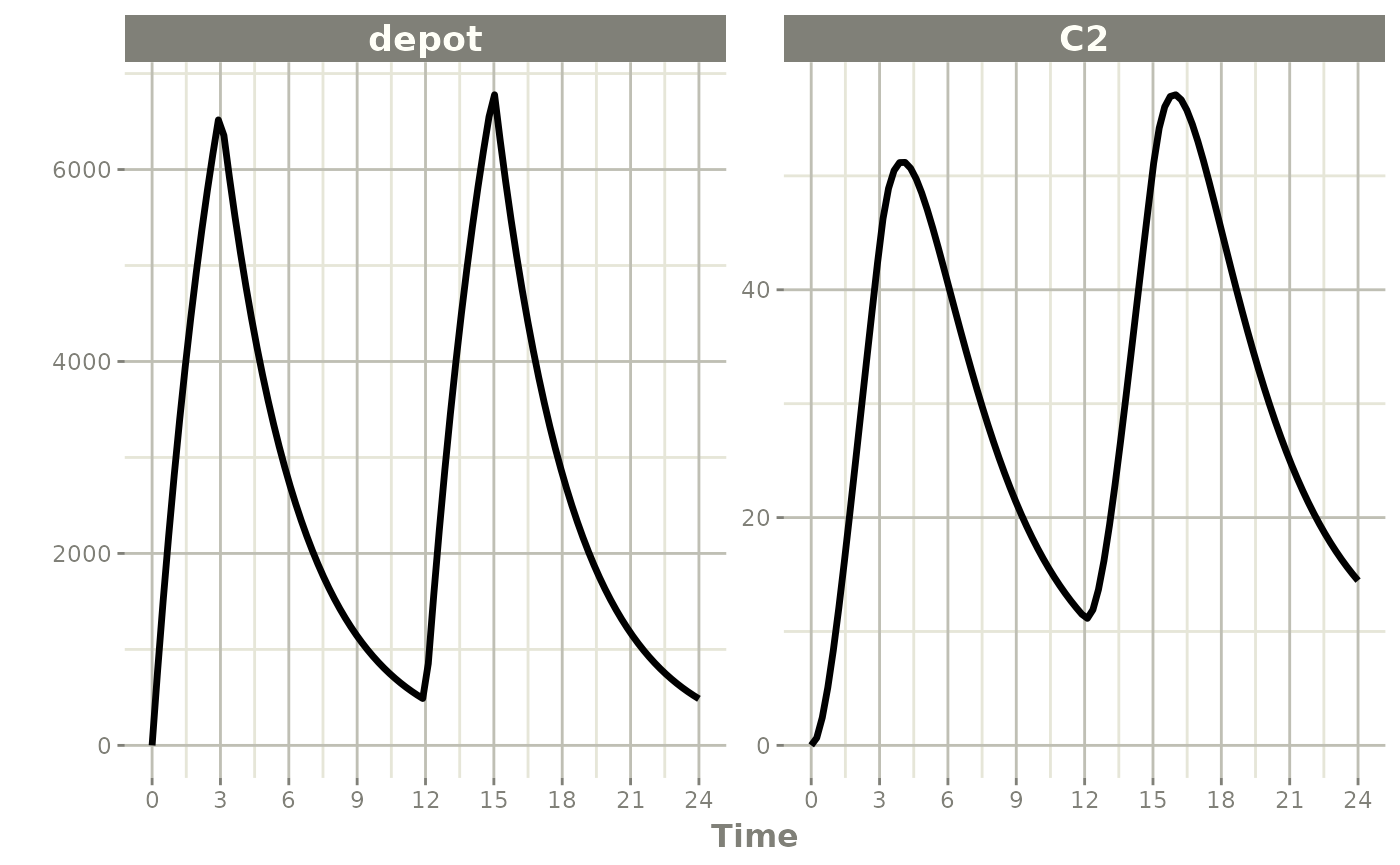

rxSolve(m1, ev, c(rateDepot=10000/3)) |> plot(depot, C2) + xlab("Time")

#> i parameter labels from comments are typically ignored in non-interactive mode

#> i Need to run with the source intact to parse comments

Steady State

Steady-state doses are solved until a constant inter-dose interval produces a repeating cycle.

ev <- et(timeUnits="hr") |>
    et(amt=10000, ii=12, ss=1) |>
    et(seq(0, 24, length.out=100))

ev

#> -- EventTable with 101 records --
#> 1 dosing records (see x$get.dosing(); add with add.dosing or et)
#> 100 observation times (see x$get.sampling(); add with add.sampling or et)
#> -- First part of x: --
#> # A tibble: 101 x 5
#>     time   amt  ii evid             ss
#>      [h] <dbl> [h] <evid>        <int>
#>  1 0        NA  NA 0:Observation    NA
#>  2 0     10000  12 1:Dose (Add)      1
#>  3 0.242    NA  NA 0:Observation    NA
#>  4 0.485    NA  NA 0:Observation    NA
#>  5 0.727    NA  NA 0:Observation    NA
#>  6 0.970    NA  NA 0:Observation    NA
#>  7 1.21     NA  NA 0:Observation    NA
#>  8 1.45     NA  NA 0:Observation    NA
#>  9 1.70     NA  NA 0:Observation    NA
#> 10 1.94     NA  NA 0:Observation    NA
#> # i 91 more rows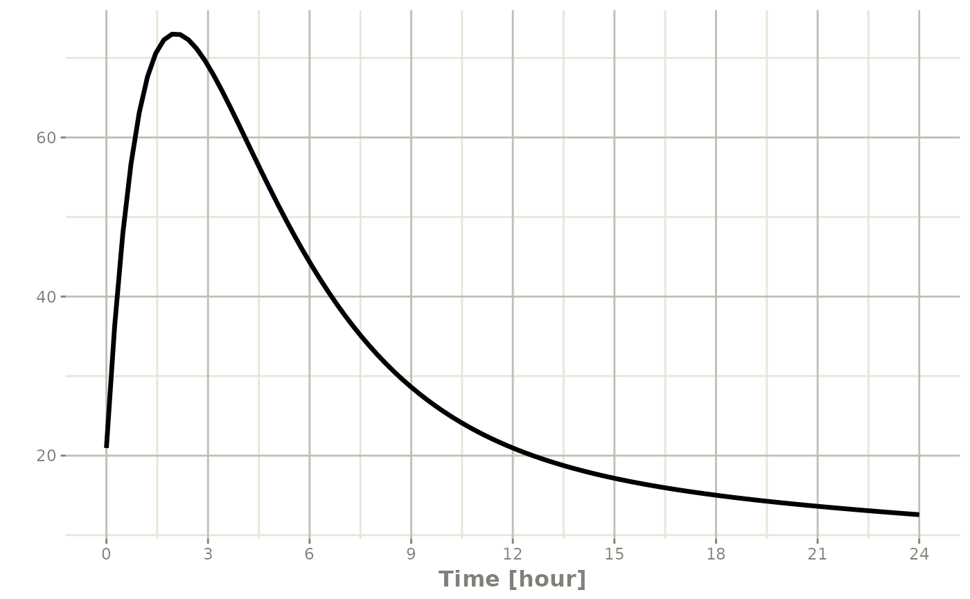

rxSolve(m1, ev) |> plot(C2)

#> i parameter labels from comments are typically ignored in non-interactive mode

#> i Need to run with the source intact to parse comments

Steady state for complex dosing (`ss=2`)

ss=2 uses superposition to achieve steady state for non-uniform dosing regimens (e.g. morning 100 mg vs evening 150 mg):

All state values are saved.
States are reset and solved to steady state.
Saved state values are added back.

ev <- et(timeUnits="hr") |>
    et(amt=10000, ii=24, ss=1) |>
    et(time=12, amt=15000, ii=24, ss=2) |>
    et(time=24, amt=10000, ii=24, addl=3) |>
    et(time=36, amt=15000, ii=24, addl=3) |>
    et(seq(0, 64, length.out=500))

library(ggplot2)

rxSolve(m1, ev, maxsteps=10000) |> plot(C2) +
  annotate("rect", xmin=0, xmax=24, ymin=-Inf, ymax=Inf, alpha=0.2) +
  annotate("text", x=12.5, y=7, label="Initial Steady State Period") +
  annotate("text", x=44,   y=7, label="Steady State AM/PM dosing")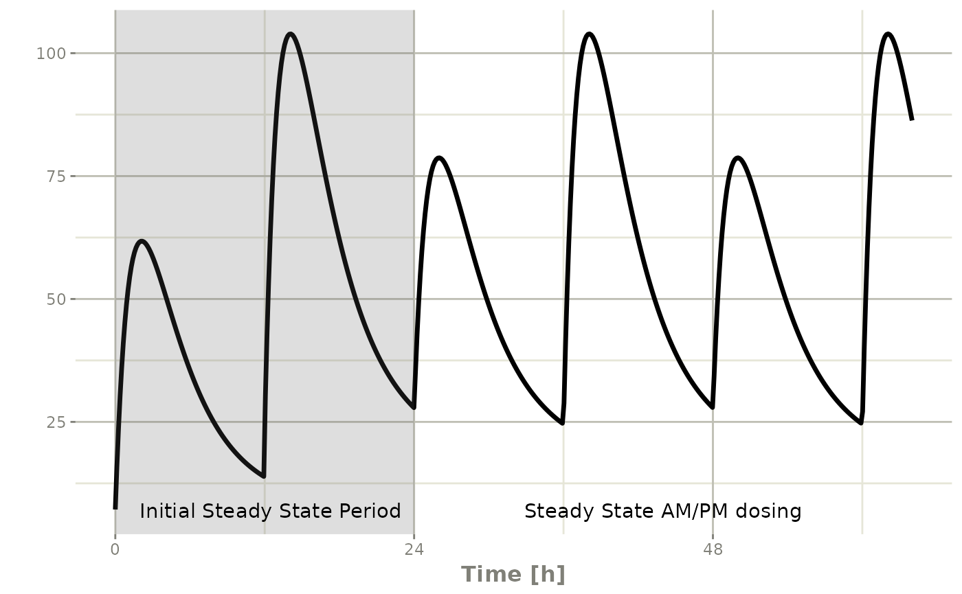

#> i parameter labels from comments are typically ignored in non-interactive mode

#> i Need to run with the source intact to parse comments

It takes a full dose cycle to reach the true complex steady-state.

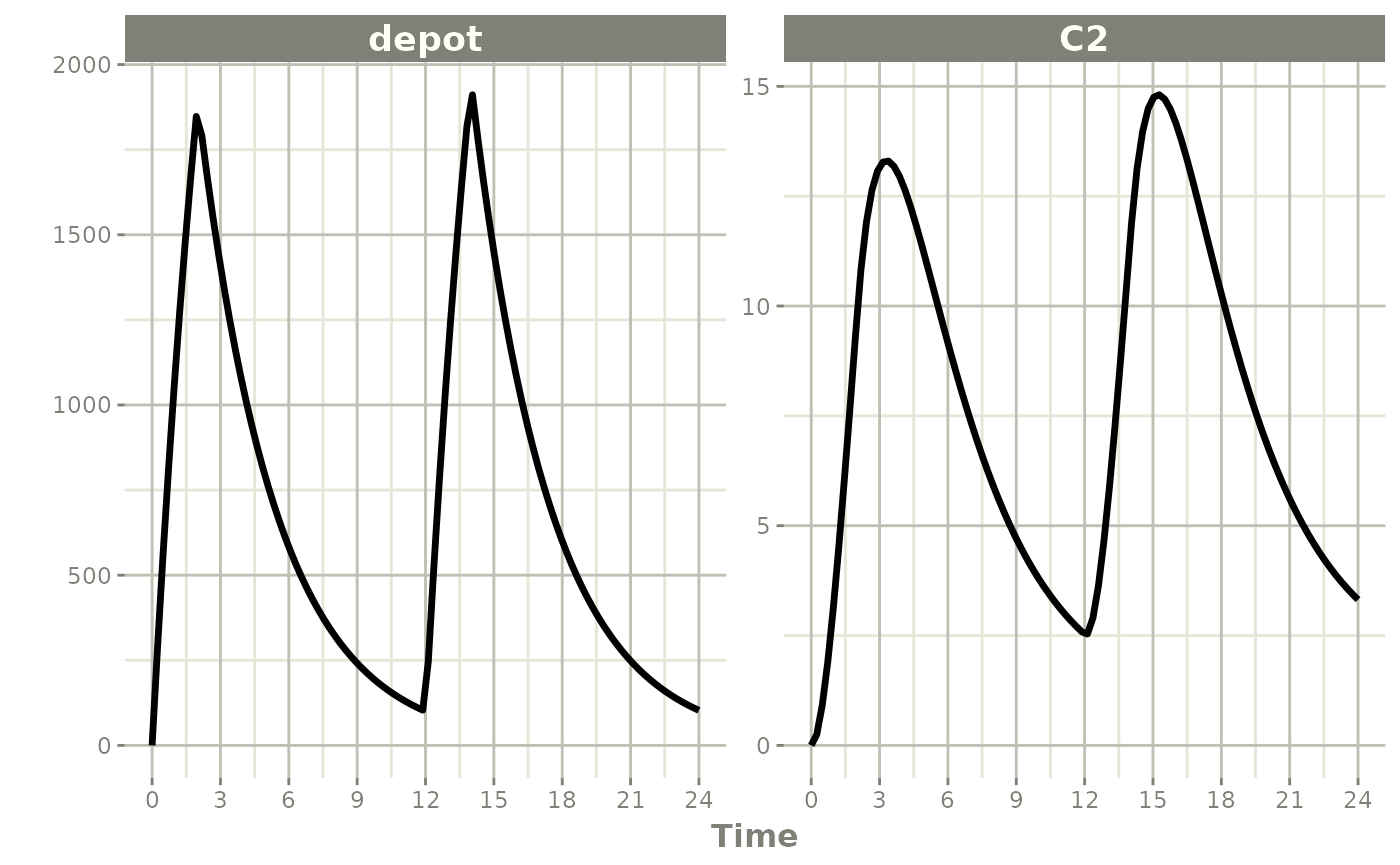
Steady state for constant infusion or zero-order processes

Constant-infusion steady state (as in NONMEM):

No inter-dose interval: ii=0
Steady-state flag: ss=1
Positive rate (rate>0) or estimated rate (rate=-1)
Zero dose: amt=0

The infusion is turned off once steady state is reached, just like NONMEM. Note that rate=-2 (modeled duration) and modeled bioavailability have no effect for this event type.

ev <- et(timeUnits="hr") |>
    et(amt=0, ss=1, rate=10000/8)

p1 <- rxSolve(m1, ev) |> plot(C2, eff)

#> i parameter labels from comments are typically ignored in non-interactive mode

#> i Need to run with the source intact to parse comments

ev <- et(timeUnits="hr") |>
    et(amt=200000, rate=10000/8) |>
    et(0, 250, length.out=1000)

p2 <- rxSolve(m1, ev) |> plot(C2, eff)

#> i parameter labels from comments are typically ignored in non-interactive mode
#> i Need to run with the source intact to parse comments

library(patchwork)
p1 / p2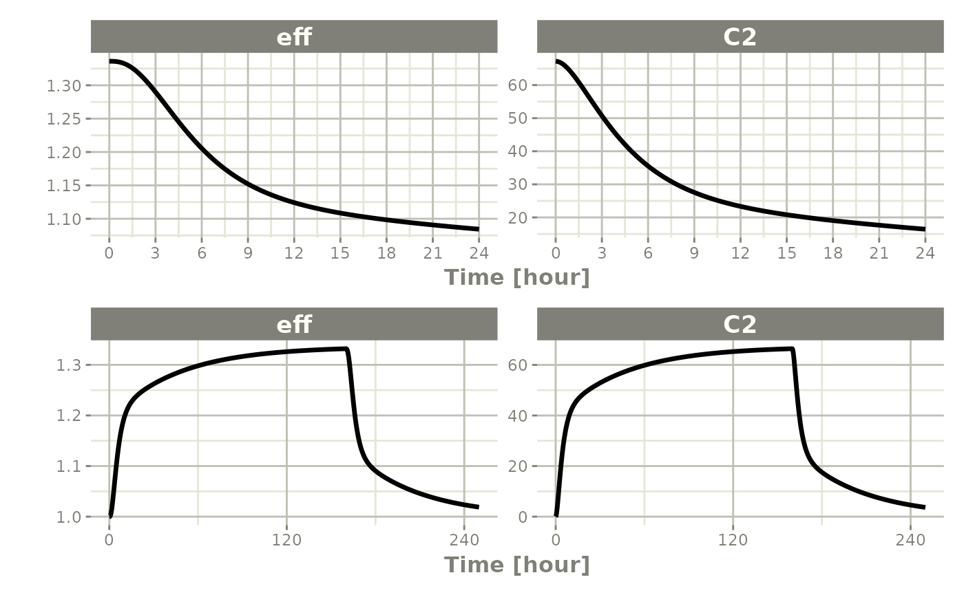

This technique can also be used for steady-state disease processes.

Reset Events

evid=3 (or evid=reset) resets all compartments to their initial values. evid=4 resets and then applies a dose.

ev <- et(timeUnits="hr") |>
    et(amt=10000, ii=12, addl=3) |>
    et(time=6, evid=reset) |>
    et(seq(0, 24, length.out=100))

ev

#> -- EventTable with 102 records --
#> 2 dosing records (see x$get.dosing(); add with add.dosing or et)
#> 100 observation times (see x$get.sampling(); add with add.sampling or et)
#> multiple doses in `addl` columns, expand with x$expand(); or etExpand(x)
#> -- First part of x: --
#> # A tibble: 102 x 5
#>     time   amt  ii  addl evid         
#>      [h] <dbl> [h] <int> <evid>       
#>  1 0        NA  NA    NA 0:Observation
#>  2 0     10000  12     3 1:Dose (Add) 
#>  3 0.242    NA  NA    NA 0:Observation
#>  4 0.485    NA  NA    NA 0:Observation
#>  5 0.727    NA  NA    NA 0:Observation
#>  6 0.970    NA  NA    NA 0:Observation
#>  7 1.21     NA  NA    NA 0:Observation
#>  8 1.45     NA  NA    NA 0:Observation
#>  9 1.70     NA  NA    NA 0:Observation
#> 10 1.94     NA  NA    NA 0:Observation
#> # i 92 more rows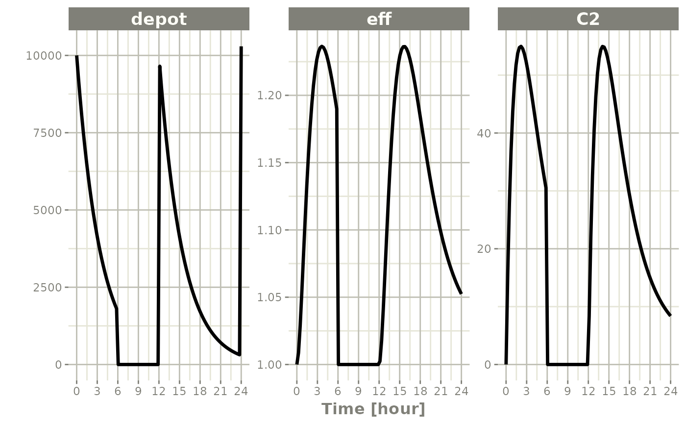

rxSolve(m1, ev) |> plot(depot, C2, eff)

#> i parameter labels from comments are typically ignored in non-interactive mode

#> i Need to run with the source intact to parse comments

All compartments are reset to their initial values at 6 hours.

ev <- et(timeUnits="hr") |>
    et(amt=10000, ii=12, addl=3) |>
    et(time=6, amt=10000, evid=4) |>
    et(seq(0, 24, length.out=100))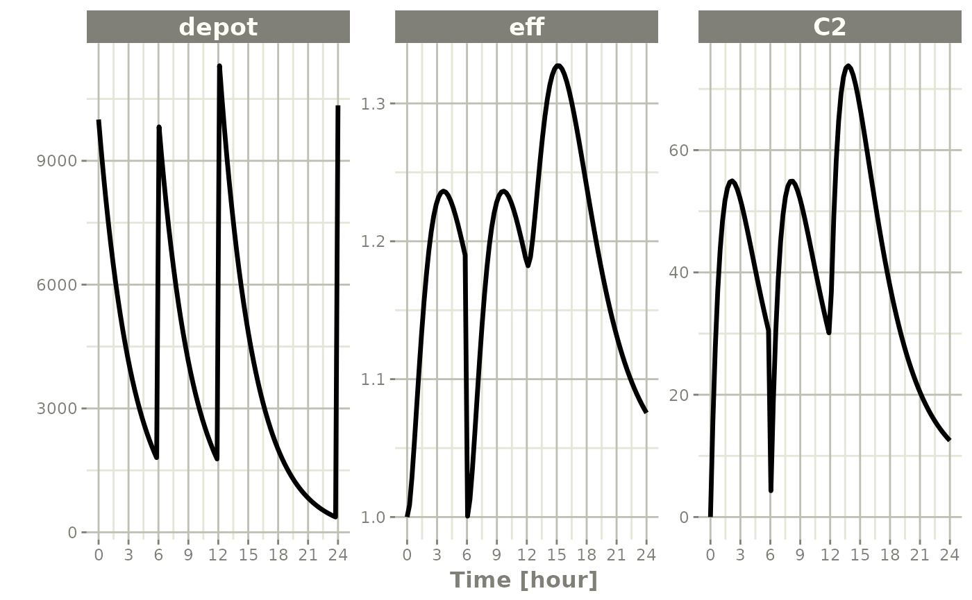

rxSolve(m1, ev) |> plot(depot, C2, eff)

#> i parameter labels from comments are typically ignored in non-interactive mode

#> i Need to run with the source intact to parse comments

Turning off compartments

Setting cmt="-depot" with evid=2 turns off a compartment: its value is set to the initial value, but other compartments are unchanged. A subsequent dose to that compartment turns it back on.

ev <- et(timeUnits="hr") |>
    et(amt=10000, ii=12, addl=3) |>
    et(time=6, cmt="-depot", evid=2) |>
    et(seq(0, 24, length.out=100))

ev

#> -- EventTable with 102 records --
#> 2 dosing records (see x$get.dosing(); add with add.dosing or et)
#> 100 observation times (see x$get.sampling(); add with add.sampling or et)
#> multiple doses in `addl` columns, expand with x$expand(); or etExpand(x)
#> -- First part of x: --
#> # A tibble: 102 x 6
#>     time cmt         amt  ii  addl evid         
#>      [h] <chr>     <dbl> [h] <int> <evid>       
#>  1 0     (obs)        NA  NA    NA 0:Observation
#>  2 0     (default) 10000  12     3 1:Dose (Add) 
#>  3 0.242 (obs)        NA  NA    NA 0:Observation
#>  4 0.485 (obs)        NA  NA    NA 0:Observation
#>  5 0.727 (obs)        NA  NA    NA 0:Observation
#>  6 0.970 (obs)        NA  NA    NA 0:Observation
#>  7 1.21  (obs)        NA  NA    NA 0:Observation
#>  8 1.45  (obs)        NA  NA    NA 0:Observation
#>  9 1.70  (obs)        NA  NA    NA 0:Observation
#> 10 1.94  (obs)        NA  NA    NA 0:Observation
#> # i 92 more rows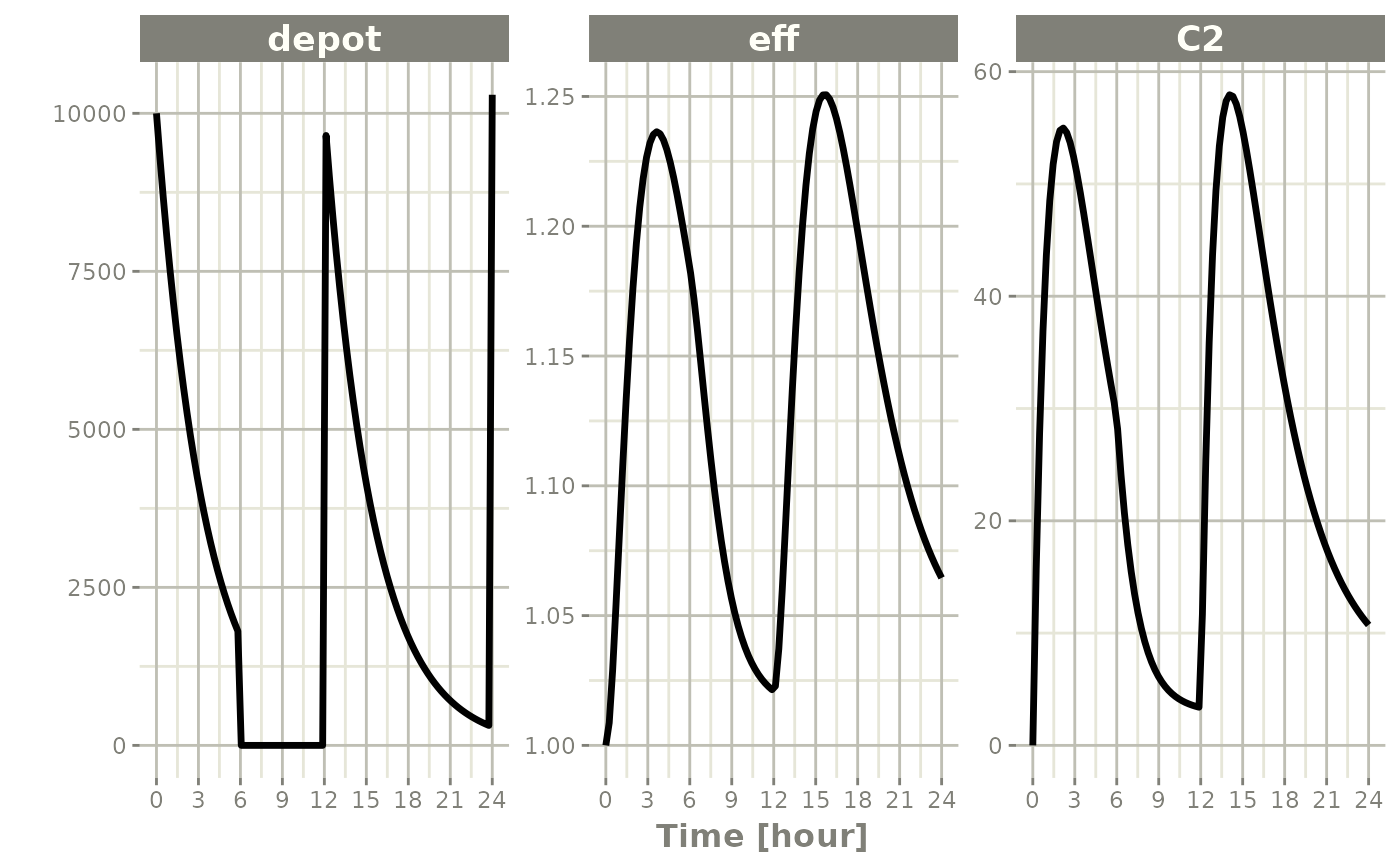

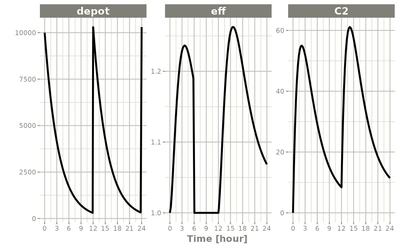
rxSolve(m1, ev) |> plot(depot, C2, eff)

#> i parameter labels from comments are typically ignored in non-interactive mode

#> i Need to run with the source intact to parse comments

Note that a dose turns back on only the compartment that was dosed. Turning off the effect compartment keeps it off even after a new depot dose:

ev <- et(timeUnits="hr") |>
    et(amt=10000, ii=12, addl=3) |>
    et(time=6, cmt="-eff", evid=2) |>
    et(seq(0, 24, length.out=100))

rxSolve(m1, ev) |> plot(depot, C2, eff)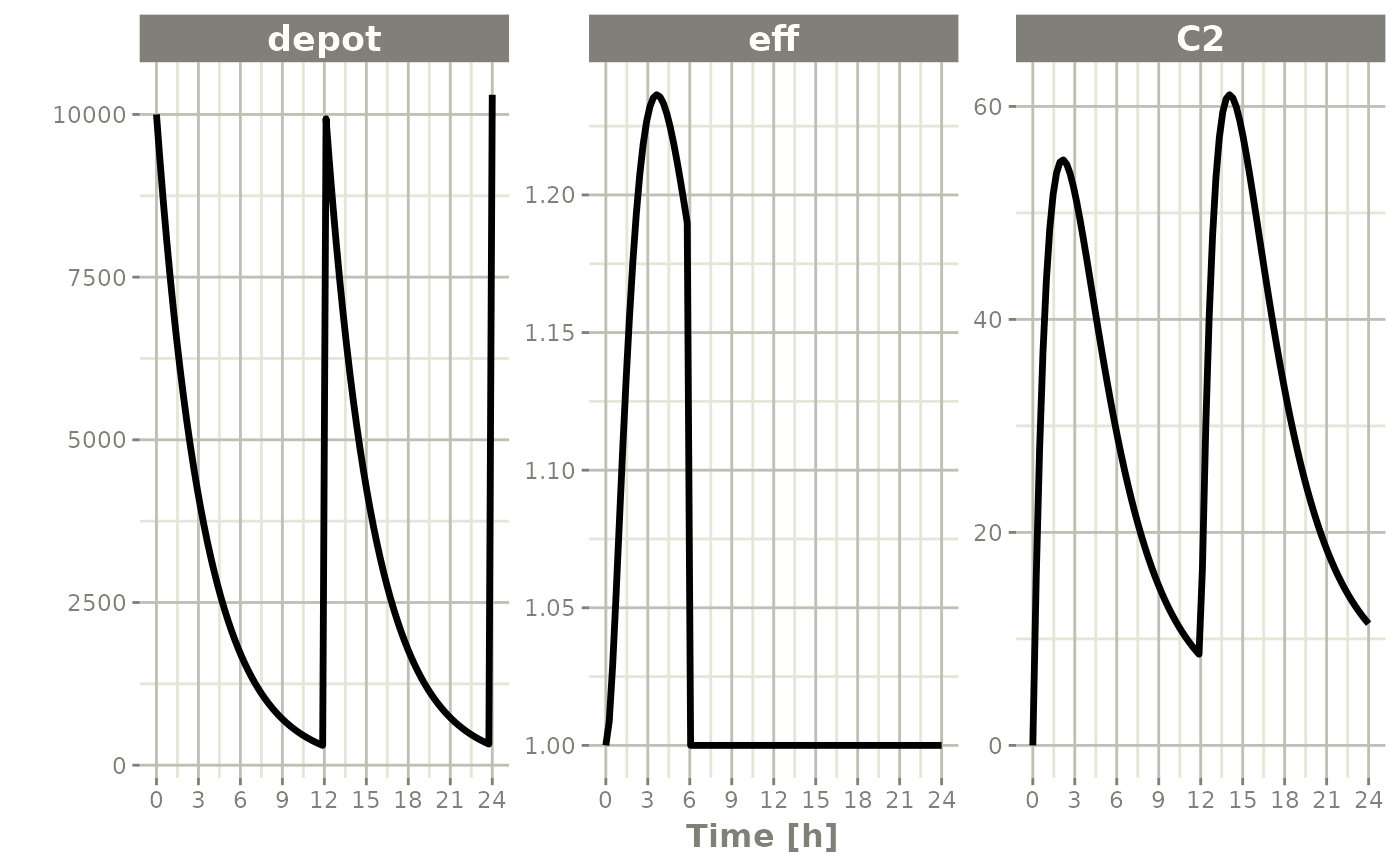

#> i parameter labels from comments are typically ignored in non-interactive mode

#> i Need to run with the source intact to parse comments

To re-enable it, send a zero dose or an evid=2 event to the compartment:

ev <- et(timeUnits="hr") |>
    et(amt=10000, ii=12, addl=3) |>
    et(time=6,  cmt="-eff", evid=2) |>
    et(time=12, cmt="eff",  evid=2) |>
    et(seq(0, 24, length.out=100))

rxSolve(m1, ev) |> plot(depot, C2, eff)

#> i parameter labels from comments are typically ignored in non-interactive mode

#> i Need to run with the source intact to parse comments

2026-04-02