Summarizing simulations with confint()

library(rxode2)
#> rxode2 5.1.7 using 2 threads (see ?getRxThreads)
#>   no cache: create with `rxCreateCache()`
library(ggplot2)

confint() turns a solved rxode2 object into the percentiles of the simulated values at each time, and – when the simulation can support it – a confidence band around each of those percentiles. This article covers what it returns, which arguments control it, and why the returned columns change with the size and structure of the simulation.

A model to summarize

pkModel <- function() {
  ini({
    tka  <- log(1.57)
    tcl  <- log(2.72)
    tv   <- log(31.07)
    eta.ka ~ 0.6
    eta.cl ~ 0.09
    eta.v  ~ 0.1
    add.sd <- 0.7
  })
  model({
    ka <- exp(tka + eta.ka)
    cl <- exp(tcl + eta.cl)
    v  <- exp(tv  + eta.v)
    d/dt(depot)  <- -ka * depot
    d/dt(center) <- ka * depot - cl / v * center
    cp <- center / v
    cp ~ add(add.sd)
  })
}

## uncertainty in the fixed effects, as it would come from the
## covariance step of an estimation run
thetaVcov <- lotri::lotri({
  tka ~ 0.04
  tcl ~ c(0.01, 0.02)
  tv  ~ 0.03
})

ev <- et(amt = 100, time = 0) |>
  et(seq(0, 24, by = 0.5))

Two levels of summary, and two shapes of output

There are two different things you may want from a simulation:

the percentiles of the population: at each time, the 2.5th, 50th and 97.5th percentile of the simulated individuals. This describes the spread of the individuals.
a confidence band around each of those percentiles: how well each percentile itself is known. This describes the uncertainty in the summary, and it is what the shaded ribbons of a visual predictive check show.

confint() returns the first as a rxSolveConfint1 object, with the percentile in p1 and its value in eff, and the second as a rxSolveConfint2 object, with the percentile in p1 and its band in the p2.5, p50 and p97.5 columns.

level sets the population percentiles. ci sets the width of the band placed around them, and defaults to level:

## 90% of the individuals, with a 95% band around each of those three curves
confint(sim, "cp", level = 0.90, ci = 0.95)

Where the band comes from

The band needs replicate estimates of the percentile. confint() gets them in one of two ways, and this is what decides which of the two shapes you get back.

`nStud > 1`: replicate studies

This is the case the band is really meant for. With thetaMat and nStud, each study is a separate draw of the fixed effects, so the percentiles are computed within each study and the band is the quantile of those study-level percentiles. The band then reflects the parameter uncertainty, which is usually what is wanted.

rxSetSeed(42)

simStud <- rxSolve(
  pkModel,
  ev,
  thetaMat = thetaVcov,  # uncertainty in the thetas
  nStud    = 500,        # virtual studies (one parameter draw each)
  nSub     = 20          # subjects per study
)
#> ℹ parameter labels from comments are typically ignored in non-interactive mode
#> ℹ Need to run with the source intact to parse comments
#> [====|====|====|====|====|====|====|====|====|====] 0:00:00

ciStud <- confint(simStud, "cp", level = 0.95)
#> ℹ this simulation drew from 'thetaMat', so the simulated values include parameter uncertainty
#> summarizing data...done

class(ciStud)[1]
#> [1] "rxSolveConfint2"

head(ciStud)
#> # A tibble: 6 × 7
#>       p1  time trt    p2.5   p50 p97.5 Percentile
#>    <dbl> <dbl> <fct> <dbl> <dbl> <dbl> <fct>     
#> 1 0.0250   0   cp    0     0      0    2.5%      
#> 2 0.5      0   cp    0     0      0    50%       
#> 3 0.975    0   cp    0     0      0    97.5%     
#> 4 0.0250   0.5 cp    0.261 0.564  1.22 2.5%      
#> 5 0.5      0.5 cp    1.02  1.66   2.63 50%       
#> 6 0.975    0.5 cp    2.23  3.65   5.71 97.5%

plot(ciStud)
#> Warning: `aes_string()` was deprecated in ggplot2 3.0.0.
#> ℹ Please use tidy evaluation idioms with `aes()`.
#> ℹ See also `vignette("ggplot2-in-packages")` for more information.
#> ℹ The deprecated feature was likely used in the rxode2 package.
#>   Please report the issue at <https://github.com/nlmixr2/rxode2/issues/>.
#> This warning is displayed once per session.
#> Call `lifecycle::last_lifecycle_warnings()` to see where this warning was
#> generated.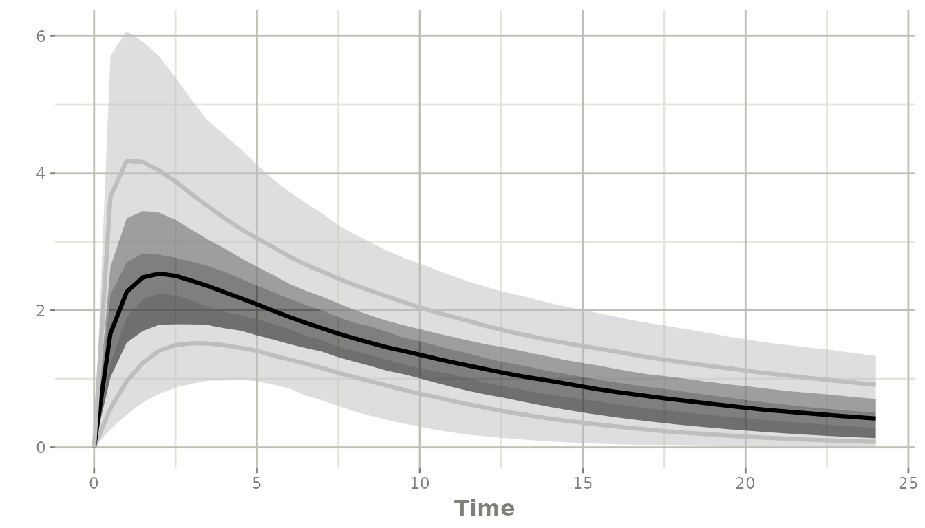

The solid line is the median individual, the ribbon around it is the 95% confidence band on that median, and the outer ribbons are the same band on the 2.5th and 97.5th percentiles.

Note that nSub = 20 subjects per study is not a problem here: the band comes from the 500 studies, not from the 20 subjects.

One study of at least 2500 individuals: sub-sampling

With a single study there are no replicates to work with, so confint() makes some: the individuals are split into round(sqrt(n)) equal sub-samples, the percentiles are computed in each, and the band is the quantile across sub-samples. This is the sampling variability of the percentile estimate itself, and it does not include any parameter uncertainty.

confint() only does this when there are at least 2500 individuals, which is the point at which the sub-samples are large enough (sqrt(2500) = 50 sub-samples of 50) for their percentiles to mean something.

rxSetSeed(42)

simBig <- rxSolve(pkModel, ev, nSub = 2500)

ciBig <- confint(simBig, "cp", level = 0.95)

class(ciBig)[1]
#> [1] "rxSolveConfint2"

head(ciBig)
#> # A tibble: 6 × 7
#>       p1  time trt    p2.5   p50 p97.5 Percentile
#>    <dbl> <dbl> <fct> <dbl> <dbl> <dbl> <fct>     
#> 1 0.0250   0   cp    0     0     0     2.5%      
#> 2 0.5      0   cp    0     0     0     50%       
#> 3 0.975    0   cp    0     0     0     97.5%     
#> 4 0.0250   0.5 cp    0.303 0.526 0.790 2.5%      
#> 5 0.5      0.5 cp    1.36  1.66  1.99  50%       
#> 6 0.975    0.5 cp    3.12  3.90  4.60  97.5%

Below 2500 individuals there is nothing to build a band from, so confint() says so and returns the percentiles alone:

rxSetSeed(42)

simSmall <- rxSolve(pkModel, ev, nSub = 2400)

ciSmall <- confint(simSmall, "cp", level = 0.95)
#> ! in order to put confidence bands around the intervals, you need at least 2500 simulations
#> summarizing data...done

class(ciSmall)[1]
#> [1] "rxSolveConfint1"

head(ciSmall)
#> # A tibble: 6 × 5
#>    time trt       p1   eff Percentile
#>   <dbl> <fct>  <dbl> <dbl> <chr>     
#> 1   0   cp    0.0250 0     2.5%      
#> 2   0   cp    0.5    0     50%       
#> 3   0   cp    0.975  0     97.5%     
#> 4   0.5 cp    0.0250 0.451 2.5%      
#> 5   0.5 cp    0.5    1.64  50%       
#> 6   0.5 cp    0.975  4.34  97.5%

This is the one surprising part of the interface: the same confint() call returns different columns for nSub = 2400 and nSub = 2500. The threshold is a property of the simulation, not of the call.

Asking for the percentiles only

If you want the simple percentiles regardless of how large the simulation is – for instance because downstream code expects fixed column names – pass ci = FALSE:

ciNone <- confint(simBig, "cp", level = 0.95, ci = FALSE)

class(ciNone)[1]
#> [1] "rxSolveConfint1"

head(ciNone)
#> # A tibble: 6 × 5
#>    time trt       p1   eff Percentile
#>   <dbl> <fct>  <dbl> <dbl> <chr>     
#> 1   0   cp    0.0250 0     2.5%      
#> 2   0   cp    0.5    0     50%       
#> 3   0   cp    0.975  0     97.5%     
#> 4   0.5 cp    0.0250 0.459 2.5%      
#> 5   0.5 cp    0.5    1.66  50%       
#> 6   0.5 cp    0.975  4.11  97.5%

ci = FALSE also pools across studies when there are several, so it gives the percentiles of all nStud * nSub simulated individuals together.

`confint()` tells you whether `thetaMat` was used

A thetaMat passed to rxSolve() is only drawn from when the variability is actually being simulated – that is, when nStud > 1, or when simVariability = TRUE forces it. With nStud = 1 it is silently ignored, so a summary of that solve carries no parameter uncertainty no matter how many individuals it has.

confint() says which of the two happened while it builds the summary:

ciStud <- confint(simStud, "cp", level = 0.95)
#> ℹ this simulation drew from 'thetaMat', so the simulated values include parameter uncertainty
#> summarizing data...done

rxSetSeed(42)

simIgnored <- rxSolve(pkModel, ev, thetaMat = thetaVcov,
                      nStud = 1, nSub = 2500)
#> Warning: 'thetaMat' is ignored since nStud <= 1
#> use 'simVariability = TRUE' to override.

ciIgnored <- confint(simIgnored, "cp", level = 0.95)
#> ! this simulation did not draw from 'thetaMat' ('nStud' <= 1), so the simulated values do not include parameter uncertainty; use 'nStud' > 1 or 'simVariability=TRUE'
#> summarizing data...done

Nothing is said when the solve had no thetaMat at all.

The message describes the simulated values, not the band. A solve can carry parameter uncertainty and still have no study dimension left to place a band with – nStud = 20, nSub = 1 gives 20 studies of one subject each, so each study percentile is that subject’s single value and a band built from them would be identical at 2.5%, 50% and 97.5%. confint() reports the pooled percentiles in that case, and those do carry the parameter uncertainty.

The two bands are not the same quantity

It is worth comparing the two directly. Both simulations below have 10000 individuals; only the second one carries parameter uncertainty.

rxSetSeed(42)
simPop <- rxSolve(pkModel, ev, nSub = 10000)
#> [====|====|====|====|====|====|====|====|====|====
ciPop <- confint(simPop, "cp", level = 0.95)

rxSetSeed(42)
simUnc <- rxSolve(pkModel, ev, thetaMat = thetaVcov,
                  nStud = 500, nSub = 20)
#> [====|====|====|====|====|====|====|====|====|====
ciUnc <- confint(simUnc, "cp", level = 0.95)

## width of the band on the median at 4 h
subset(as.data.frame(ciPop), time == 4 & p1 == 0.5, c("p2.5", "p50", "p97.5"))
#>        p2.5      p50    p97.5
#> 26 2.153695 2.283792 2.418434
subset(as.data.frame(ciUnc), time == 4 & p1 == 0.5, c("p2.5", "p50", "p97.5"))
#>        p2.5      p50    p97.5
#> 26 1.737957 2.263534 2.903909

The sub-sampled band is much narrower: with the parameters held fixed, 10000 individuals pin the population median down tightly. The band from the replicate studies is wider because the thetas themselves are only known to within thetaVcov. If you want a band that means “how well do we know this curve”, simulate with thetaMat/nStud; the sub-sampled band answers the narrower question “how much would this curve move if we re-drew the individuals”.

Stratifying with `by`

Columns carried through the solve with keep= can be used to split the summary:

evDose <- rbind(
  data.frame(et(amt = 100, time = 0) |> et(seq(0, 24, by = 2)) |>
               et(id = 1:100), dose = 100),
  data.frame(et(amt = 300, time = 0) |> et(seq(0, 24, by = 2)) |>
               et(id = 101:200), dose = 300)
)

rxSetSeed(42)
simBy <- rxSolve(pkModel, evDose, keep = "dose")

ciBy <- confint(simBy, "cp", level = 0.95, by = "dose")

head(ciBy)
#> # A tibble: 6 × 6
#>    time trt    dose     p1   eff Percentile
#>   <dbl> <fct> <dbl>  <dbl> <dbl> <chr>     
#> 1     0 cp      100 0.0250  0    2.5%      
#> 2     0 cp      100 0.5     0    50%       
#> 3     0 cp      100 0.975   0    97.5%     
#> 4     2 cp      100 0.0250  1.23 2.5%      
#> 5     2 cp      100 0.5     2.49 50%       
#> 6     2 cp      100 0.975   4.23 97.5%

Means instead of percentiles

mean = TRUE reports the mean and its confidence interval with meanProbs() rather than the empirical quantiles, and mean = "binom" uses binomProbs() for a 0/1 variable such as a target-attainment indicator:

head(confint(simSmall, "cp", level = 0.95, mean = TRUE))
#> # A tibble: 6 × 5
#>    time trt       p1   eff Percentile
#>   <dbl> <fct>  <dbl> <dbl> <chr>     
#> 1   0   cp    0.0250  0    2.5%      
#> 2   0   cp    0.5     0    50%       
#> 3   0   cp    0.975   0    97.5%     
#> 4   0.5 cp    0.0250  1.78 2.5%      
#> 5   0.5 cp    0.5     1.82 50%       
#> 6   0.5 cp    0.975   1.86 97.5%

Summary

Simulation	`confint()` returns
any, with `ci = FALSE`	percentiles only (`p1`, `eff`)
`nStud > 1`	percentiles per study, band across studies (`p1`, `p2.5`, `p50`, `p97.5`)
one study, `>= 2500` individuals	percentiles per sub-sample, band across sub-samples
one study, `< 2500` individuals	percentiles only, with a message

See also the parameter uncertainty article for how to build the thetaMat/nStud simulation the band is meant for, and the VPC article for the diagnostic version of the same idea.