Setting up the rxode2 model for the pipeline
In this example we will show how to use rxode2 in a simple pipeline.
We can start with a model that can be used for the different simulation workflows that rxode2 can handle:
library(rxode2)
#> rxode2 5.1.3 using 2 threads (see ?getRxThreads)
#>   no cache: create with `rxCreateCache()`

Ribba2012 <- function() {
  ini({
    k = 100
    tkde = 0.24
    eta.tkde = 0
    tkpq = 0.0295
    eta.kpq = 0
    tkqpp = 0.0031
    eta.kqpp = 0
    tlambdap = 0.121
    eta.lambdap = 0
    tgamma = 0.729
    eta.gamma = 0
    tdeltaqp = 0.00867
    eta.deltaqp = 0
    prop.sd <- 0
    tpt0 = 7.13
    eta.pt0 = 0
    tq0 = 41.2
    eta.q0 = 0
  })
  model({
    kde ~ tkde*exp(eta.tkde)
    kpq ~ tkpq * exp(eta.kpq)
    kqpp ~ tkqpp * exp(eta.kqpp)
    lambdap ~ tlambdap*exp(eta.lambdap)
    gamma ~ tgamma*exp(eta.gamma)
    deltaqp ~ tdeltaqp*exp(eta.deltaqp)
    d/dt(c) = -kde * c
    d/dt(pt) = lambdap * pt *(1-pstar/k) + kqpp*qp -
      kpq*pt - gamma*c*kde*pt
    d/dt(q) = kpq*pt -gamma*c*kde*q
    d/dt(qp) = gamma*c*kde*q - kqpp*qp - deltaqp*qp
    ## initial conditions
    pt0 ~ tpt0*exp(eta.pt0)
    q0 ~ tq0*exp(eta.q0)
    pt(0) = pt0
    q(0) = q0
    pstar <- (pt+q+qp)
    pstar ~  prop(prop.sd)
  })
}
This is a tumor growth model described in Ribba 2012. In this case,
we compiled the model into an R object Ribba2012, though in
an rxode2 simulation pipeline, you do not have to assign the
compiled model to any object, though I think it makes sense.
Simulating one event table
Simulating a single event table is quite simple:
- You pipe the rxode2 simulation object into an event table object by
et(). - When the events are completely specified, you simply solve the ODE
system with
rxSolve(). - In this case you can pipe the output to
plot()to conveniently view the results. - Note for the plot we are only selecting the selecting following:
-
pt(Proliferative Tissue), -
q(quiescent tissue) -
qp(DNA-Damaged quiescent tissue) and -
pstar(total tumor tissue)
-
Ribba2012 |> # Use rxode2
    et(time.units="months") |> # Pipe to a new event table
    et(amt=1, time=50, until=58, ii=1.5) |> # Add dosing every 1.5 months
    et(0, 250, by=0.5) |> # Add some sampling times (not required)
    rxSolve() |> # Solve the simulation
    plot(pt, q, qp, pstar) # Plot it, plotting the variables of interest
#> ℹ parameter labels from comments are typically ignored in non-interactive mode
#> ℹ Need to run with the source intact to parse comments
#> ℹ parameter labels from comments are typically ignored in non-interactive mode
#> ℹ Need to run with the source intact to parse comments
#> ℹ parameter labels from comments are typically ignored in non-interactive mode
#> ℹ Need to run with the source intact to parse comments
#> ℹ parameter labels from comments are typically ignored in non-interactive mode
#> ℹ Need to run with the source intact to parse comments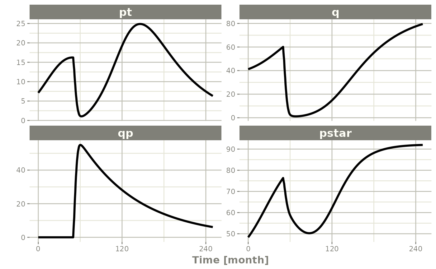
Simulating multiple subjects from a single event table
Simulating with between subject variability
The next sort of simulation that may be useful is simulating multiple
patients with the same treatments. In this case, we will use the
omega matrix specified by the paper:
## Add CVs from paper for individual simulation
## Uses exact formula:

lognCv = function(x){log((x/100)^2+1)}

library(lotri)
## Now create omega matrix
## I'm using lotri to quickly specify names/diagonals
omega <- lotri(eta.pt0 ~ lognCv(94),
               eta.q0 ~ lognCv(54),
               eta.lambdap ~ lognCv(72),
               eta.kqp ~ lognCv(76),
               eta.kqpp ~ lognCv(97),
               eta.deltaqp ~ lognCv(115),
               eta.tkde ~ lognCv(70))

omega
#>               eta.pt0    eta.q0 eta.lambdap   eta.kqp  eta.kqpp eta.deltaqp
#> eta.pt0     0.6331848 0.0000000   0.0000000 0.0000000 0.0000000   0.0000000
#> eta.q0      0.0000000 0.2558818   0.0000000 0.0000000 0.0000000   0.0000000
#> eta.lambdap 0.0000000 0.0000000   0.4176571 0.0000000 0.0000000   0.0000000
#> eta.kqp     0.0000000 0.0000000   0.0000000 0.4559047 0.0000000   0.0000000
#> eta.kqpp    0.0000000 0.0000000   0.0000000 0.0000000 0.6631518   0.0000000
#> eta.deltaqp 0.0000000 0.0000000   0.0000000 0.0000000 0.0000000   0.8426442
#> eta.tkde    0.0000000 0.0000000   0.0000000 0.0000000 0.0000000   0.0000000
#>              eta.tkde
#> eta.pt0     0.0000000
#> eta.q0      0.0000000
#> eta.lambdap 0.0000000
#> eta.kqp     0.0000000
#> eta.kqpp    0.0000000
#> eta.deltaqp 0.0000000
#> eta.tkde    0.3987761
With this information, it is easy to simulate 3 subjects from the model-based parameters:
set.seed(1089)
rxSetSeed(1089)
Ribba2012 |> # Use rxode2
    et(time.units="months") |> # Pipe to a new event table
    et(amt=1, time=50, until=58, ii=1.5) |> # Add dosing every 1.5 months
    et(0, 250, by=0.5) |> # Add some sampling times (not required)
    rxSolve(nSub=3, omega=omega) |> # Solve the simulation
    plot(pt, q, qp, pstar) # Plot it, plotting the variables of interest
#> ℹ parameter labels from comments are typically ignored in non-interactive mode
#> ℹ Need to run with the source intact to parse comments
#> ℹ parameter labels from comments are typically ignored in non-interactive mode
#> ℹ Need to run with the source intact to parse comments
#> ℹ parameter labels from comments are typically ignored in non-interactive mode
#> ℹ Need to run with the source intact to parse comments
#> Warning: multi-subject simulation without without 'omega'
Note there are two different things that were added to this
simulation: - nSub to specify how many subjects are in the
model - omega to specify the between subject
variability.
Simulation with unexplained variability
You can even add unexplained variability quite easily:
Ribba2012 |> # Use rxode2
  ini(prop.sd=0.05) |> # change variability
  et(time.units="months") |> # Pipe to a new event table
  et(amt=1, time=50, until=58, ii=1.5) |> # Add dosing every 1.5 months
  et(0, 250, by=0.5) |> # Add some sampling times (not required)
  rxSolve(nSub=3, omega=omega) |>
  plot(pt, q, qp, sim) # Plot it, plotting the variables of interest
#> ℹ parameter labels from comments are typically ignored in non-interactive mode
#> ℹ Need to run with the source intact to parse comments
#> ℹ change initial estimate of `prop.sd` to `0.05`
#> Warning: multi-subject simulation without without 'omega'
# note that sim is the simulated pstar since this is simulated from the
# model with a nlmixr2 endpoint
In this case we only added the sigma matrix to have
unexplained variability on the pstar or total tumor
tissue.
You can even simulate with uncertainty in the theta
omega and sigma values if you wish.
Simulation with uncertainty in all the parameters (by matrices)
If we assume these parameters came from 95 subjects with
8 observations apiece, the degrees of freedom for the omega
matrix would be 95, and the degrees of freedom of the
sigma matrix would be 95*8=760 because
95 items informed the omega matrix, and
760 items informed the sigma matrix.
Ribba2012 |> # Use rxode2
  ini(prop.sd = 0.05) |>
  et(time.units="months") |> # Pipe to a new event table
  et(amt=1, time=50, until=58, ii=1.5) |> # Add dosing every 1.5 months
  et(0, 250, by=0.5) |> # Add some sampling times (not required)
  rxSolve(nSub=3, nStud=3, omega=omega,
          dfSub=760, dfObs=95) |> # Solve the simulation
  plot(pt, q, qp, sim) # Plot it, plotting the variables of interest
#> ℹ parameter labels from comments are typically ignored in non-interactive mode
#> ℹ Need to run with the source intact to parse comments
#> ℹ change initial estimate of `prop.sd` to `0.05`
#> Warning: multi-subject simulation without without 'omega'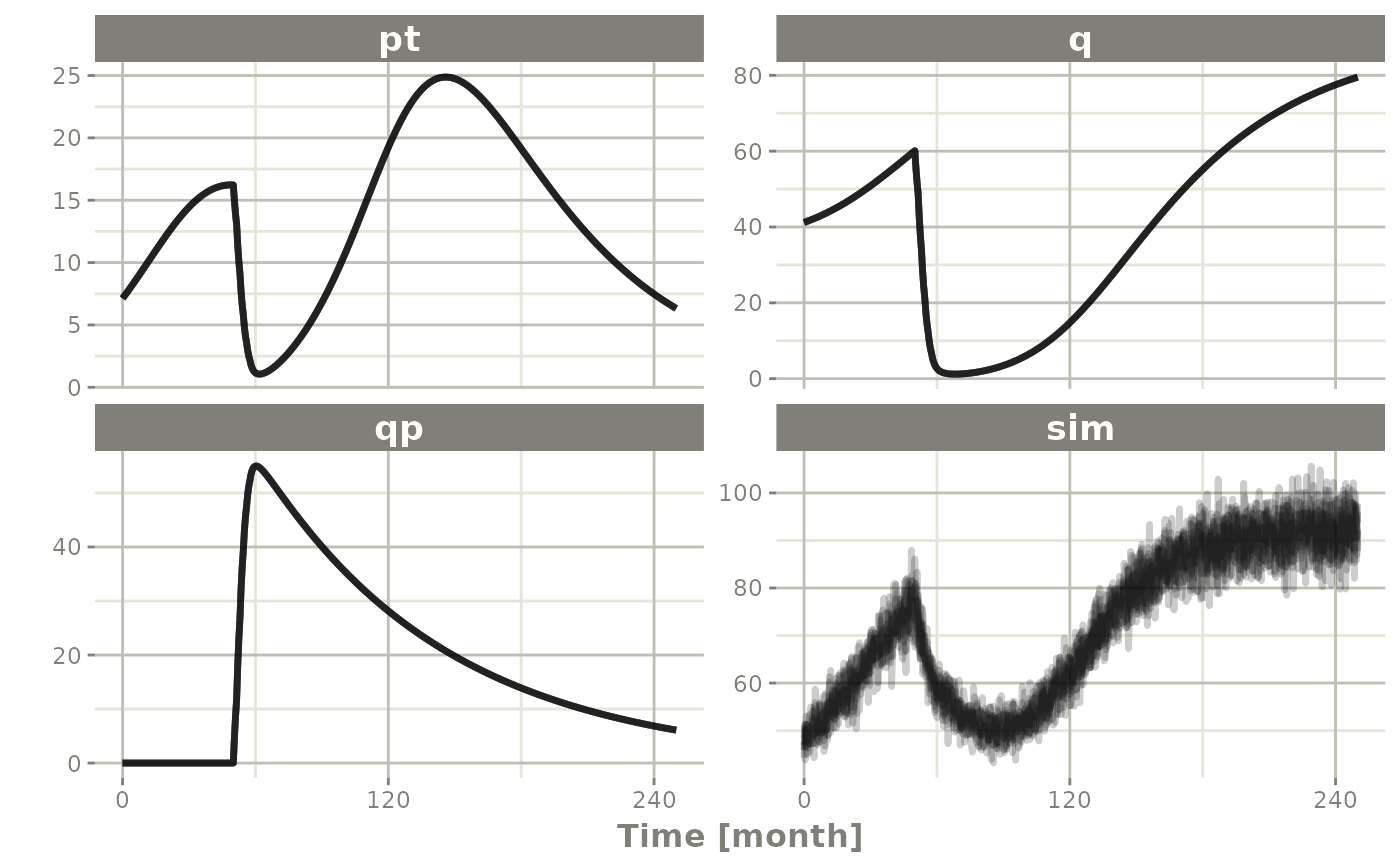
Often in simulations we have a full covariance matrix for the fixed
effect parameters. In this case, we do not have the matrix, but it could
be specified by thetaMat.
While we do not have a full covariance matrix, we can have information about the diagonal elements of the covariance matrix from the model paper. These can be converted as follows:
rseVar <- function(est, rse){
  return(est*rse/100)^2
}

thetaMat <- lotri(tpt0 ~ rseVar(7.13,25),
                  tq0 ~ rseVar(41.2,7),
                  tlambdap ~ rseVar(0.121, 16),
                  tkqpp ~ rseVar(0.0031, 35),
                  tdeltaqp ~ rseVar(0.00867, 21),
                  tgamma ~ rseVar(0.729, 37),
                  tkde ~ rseVar(0.24, 33)
                  )

thetaMat
#>            tpt0   tq0 tlambdap    tkqpp  tdeltaqp  tgamma   tkde
#> tpt0     1.7825 0.000  0.00000 0.000000 0.0000000 0.00000 0.0000
#> tq0      0.0000 2.884  0.00000 0.000000 0.0000000 0.00000 0.0000
#> tlambdap 0.0000 0.000  0.01936 0.000000 0.0000000 0.00000 0.0000
#> tkqpp    0.0000 0.000  0.00000 0.001085 0.0000000 0.00000 0.0000
#> tdeltaqp 0.0000 0.000  0.00000 0.000000 0.0018207 0.00000 0.0000
#> tgamma   0.0000 0.000  0.00000 0.000000 0.0000000 0.26973 0.0000
#> tkde     0.0000 0.000  0.00000 0.000000 0.0000000 0.00000 0.0792
Now we have a thetaMat to represent the uncertainty in
the theta matrix, as well as the other pieces in the
simulation. Typically you can put this information into your simulation
with the thetaMat matrix.
With such large variability in theta it is easy to
sample a negative rate constant, which does not make sense. For
example:
Ribba2012 |> # Use rxode2
ini(prop.sd = 0.05) |>
et(time.units="months") |> # Pipe to a new event table
et(amt=1, time=50, until=58, ii=1.5) |> # Add dosing every 1.5 months
et(0, 250, by=0.5) |> # Add some sampling times (not required)
rxSolve(nSub=2, nStud=2, omega=omega,
thetaMat=thetaMat,
dfSub=760, dfObs=95) |> # Solve the simulation
plot(pt, q, qp, pstar) # Plot it, plotting the variables of interest

#> ℹ change initial estimate of `prop.sd` to `0.05`
#> unhandled error message: EE:[lsoda] 70000 steps taken before reaching tout
#> @(lsoda.c:750
#> Warning message:
#> In rxSolve_(object, .ctl, .nms, .xtra, params, events, inits, setupOnly = .setupOnly) :
#>  Some ID(s) could not solve the ODEs correctly; These values are replaced with NA.
To correct these problems you simply need to use a truncated
multivariate normal and specify the reasonable ranges for the
parameters. For theta this is specified by
thetaLower and thetaUpper. Similar parameters
are there for the other matrices: omegaLower,
omegaUpper, sigmaLower and
sigmaUpper. These may be named vectors, one numeric value,
or a numeric vector matching the number of parameters specified in the
thetaMat matrix.
In this case the simulation simply has to be modified to have
thetaLower=0 to make sure all rates are positive:
Ribba2012 |> # Use rxode2
  ini(prop.sd = 0.05) |>
  et(time.units="months") |> # Pipe to a new event table
  et(amt=1, time=50, until=58, ii=1.5) |> # Add dosing every 1.5 months
  et(0, 250, by=0.5) |> # Add some sampling times (not required)
  rxSolve(nSub=2, nStud=2, omega=omega,
          thetaMat=thetaMat,
          thetaLower=0, # Make sure the rates are reasonable
          dfSub=760, dfObs=95) |> # Solve the simulation
  plot(pt, q, qp, sim) # Plot it, plotting the variables of interest
#> ℹ parameter labels from comments are typically ignored in non-interactive mode
#> ℹ Need to run with the source intact to parse comments
#> ℹ change initial estimate of `prop.sd` to `0.05`
#> Warning: multi-subject simulation without without 'omega'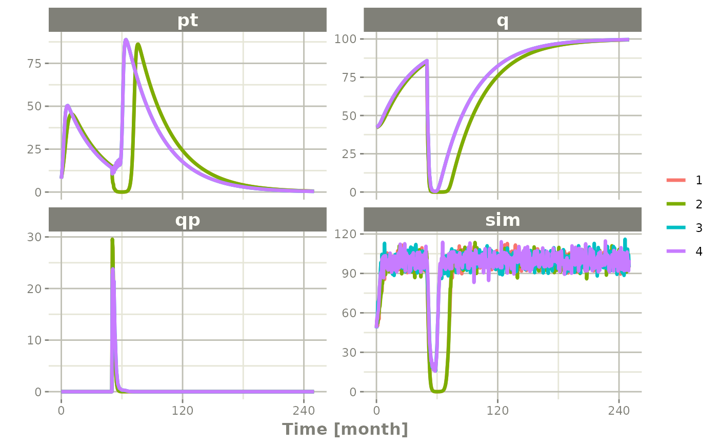
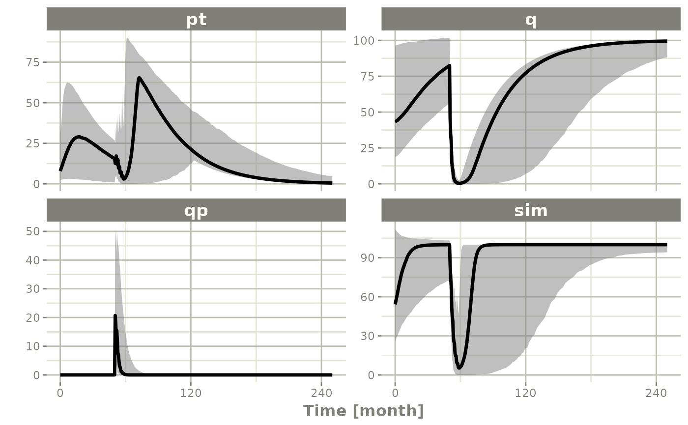
Summarizing the simulation output
While it is easy to use dplyr and
data.table to perform your own summary of simulations,
rxode2 also provides this ability by the
confint function.
## This takes a little more time; Most of the time is the summary
## time.

sim0 <- Ribba2012 |> # Use rxode2
  ini(prop.sd=0.05) |>
  et(time.units="months") |> # Pipe to a new event table
  et(amt=1, time=50, until=58, ii=1.5) |> # Add dosing every 1.5 months
  et(0, 250, by=0.5) |> # Add some sampling times (not required)
  rxSolve(nSub=10, nStud=10, omega=omega,
          thetaMat=thetaMat,
          thetaLower=0, # Make sure the rates are reasonable
          dfSub=760, dfObs=95) |> # Solve the simulation
  confint(c("pt","q","qp","sim"),level=0.90); # Create Simulation intervals
#> ℹ parameter labels from comments are typically ignored in non-interactive mode
#> ℹ Need to run with the source intact to parse comments
#> ℹ change initial estimate of `prop.sd` to `0.05`
#> Warning: multi-subject simulation without without 'omega'
#> ! in order to put confidence bands around the intervals, you need at least 2500 simulations
#> summarizing data...done

sim0 |> plot() # Plot the simulation intervals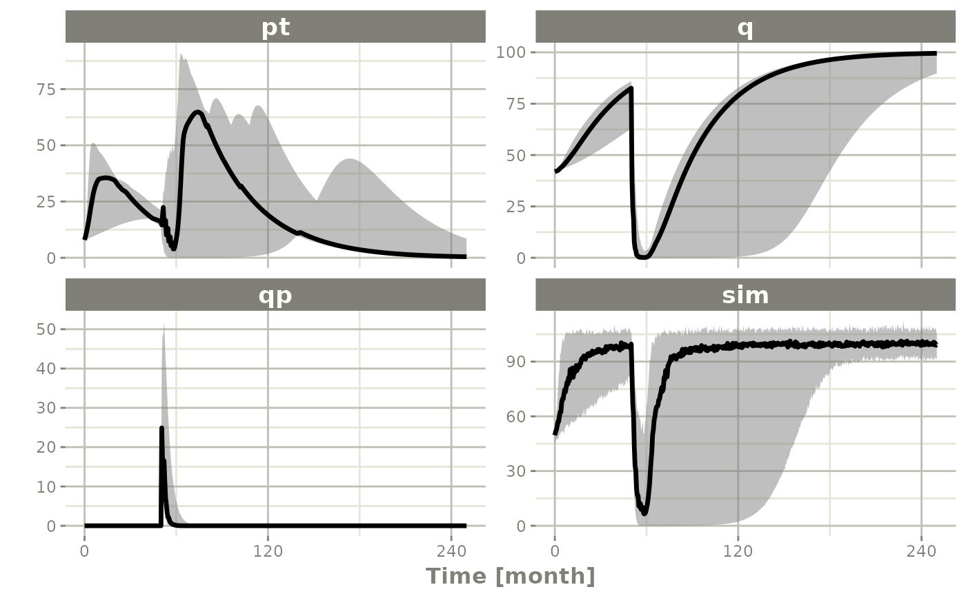
Simulating from a data-frame of parameters
While the simulation from matrices can be very useful and a fast way
to simulate information, sometimes you may want to simulate more complex
scenarios. For instance, there may be some reason to believe that
tkde needs to be above tlambdap, therefore
these need to be simulated more carefully. You can generate the data
frame in whatever way you want. The internal method of simulating the
new parameters is exported too.
library(dplyr)
#>
#> Attaching package: 'dplyr'
#> The following objects are masked from 'package:stats':
#>
#>     filter, lag
#> The following objects are masked from 'package:base':
#>
#>     intersect, setdiff, setequal, union

Ribba2012 <- Ribba2012()
# Convert to classic rxode2 model with ini attached

r <- Ribba2012$simulationIniModel

pars <- rxInits(r)
pars <- pars[regexpr("(prop|eta)",names(pars)) == -1]
print(pars)
#>           k        tkde        tkpq       tkqpp    tlambdap      tgamma
#>    1.00e+02    2.40e-01    2.95e-02    3.10e-03    1.21e-01    7.29e-01
#>    tdeltaqp        tpt0         tq0 rxerr.pstar
#>    8.67e-03    7.13e+00    4.12e+01    1.00e+00
## This is the exported method for simulation of Theta/Omega internally in rxode2
df <- rxSimThetaOmega(params=pars, omega=omega,dfSub=760,
                      thetaMat=thetaMat, thetaLower=0, nSub=60,nStud=60) |>
    filter(tkde > tlambdap) |> as_tibble()
## You could also simulate more and bind them together to a data frame.
print(df)
#> # A tibble: 2,100 × 17
#>        k  tkde   tkpq tkqpp tlambdap tgamma tdeltaqp  tpt0   tq0 rxerr.pstar
#>    <dbl> <dbl>  <dbl> <dbl>    <dbl>  <dbl>    <dbl> <dbl> <dbl>       <dbl>
#>  1   100 0.468 0.0295 0.805    0.288  0.980    0.256  8.54  41.4           1
#>  2   100 0.468 0.0295 0.805    0.288  0.980    0.256  8.54  41.4           1
#>  3   100 0.468 0.0295 0.805    0.288  0.980    0.256  8.54  41.4           1
#>  4   100 0.468 0.0295 0.805    0.288  0.980    0.256  8.54  41.4           1
#>  5   100 0.468 0.0295 0.805    0.288  0.980    0.256  8.54  41.4           1
#>  6   100 0.468 0.0295 0.805    0.288  0.980    0.256  8.54  41.4           1
#>  7   100 0.468 0.0295 0.805    0.288  0.980    0.256  8.54  41.4           1
#>  8   100 0.468 0.0295 0.805    0.288  0.980    0.256  8.54  41.4           1
#>  9   100 0.468 0.0295 0.805    0.288  0.980    0.256  8.54  41.4           1
#> 10   100 0.468 0.0295 0.805    0.288  0.980    0.256  8.54  41.4           1
#> # ℹ 2,090 more rows
#> # ℹ 7 more variables: eta.pt0 <dbl>, eta.q0 <dbl>, eta.lambdap <dbl>,
#> #   eta.kqp <dbl>, eta.kqpp <dbl>, eta.deltaqp <dbl>, eta.tkde <dbl>
## Quick check to make sure that all the parameters are OK.
all(df$tkde>df$tlambdap)
#> [1] TRUE
sim1 <- r |> # Use rxode2
    et(time.units="months") |> # Pipe to a new event table
    et(amt=1, time=50, until=58, ii=1.5) |> # Add dosing every 1.5 months
    et(0, 250, by=0.5) |> # Add some sampling times (not required)
    rxSolve(df)
## Note this information looses information about which ID is in a
## "study", so it summarizes the confidence intervals by dividing the
## subjects into sqrt(#subjects) subjects and then summarizes the
## confidence intervals
sim2 <- sim1 |> confint(c("pt","q","qp","sim"),level=0.90); # Create Simulation intervals
#> ! in order to put confidence bands around the intervals, you need at least 2500 simulations
#> summarizing data...done
save(sim2, file = file.path(system.file(package = "rxode2"), "pipeline-sim2.rds"), version = 2)
sim2 |> plot()