
Simulating time-to-event endpoints
Source:vignettes/articles/rxode2-time-to-event.Rmd
rxode2-time-to-event.Rmd
library(rxode2)
#> rxode2 5.1.8.9000 using 2 threads (see ?getRxThreads)
#>   no cache: create with `rxCreateCache()`
Hazard-based endpoints
A time-to-event (TTE) endpoint is described by its hazard
h(t), the instantaneous event rate given that no event has
happened yet. The survival since the last event is
S(t) = exp(-(H(t) - H(t_last))), where H is
the cumulative hazard. In rxode2 the endpoint is written with
tte(), following the options of Monolix’s
{type=event} definition:
seizure <- function() {
  ini({
    tcl <- log(1)
    tv <- log(10)
    eta.cl ~ 0.1
    add.sd <- 0.1
    lambda <- 0.01
    beta <- 0.1
  })
  model({
    cl <- exp(tcl + eta.cl)
    v <- exp(tv)
    d/dt(central) <- -cl / v * central
    cp <- central / v
    haz <- lambda * exp(beta * cp)
    cp ~ add(add.sd)
    ev ~ tte(haz, maxEventNumber = 1)
  })
}
The cumulative hazard is added as a hidden state
(rx.tteH.ev), and each event time solves
H(t) - H(t_last) = -log(u) with a root finder, so the event
times are exact rather than limited to the sampling grid.
Simulated rows
The endpoint’s records in the event table define each subject’s
observation window. The simulation replaces them with the rows a Monolix
or NONMEM time-to-event data set has: sim = 0 at the start
of the window, sim = 1 at each event and
sim = 0 at right censoring.
e <- et(amt = 100, cmt = "central") |>
  et(seq(0, 48, by = 4), cmt = "cp") |>
  et(c(0, 48), cmt = "ev") |>
  et(id = 1:200)

s <- withr::with_seed(42, rxSolve(seizure(), e))
tte <- as.data.frame(s)
tte <- tte[tte$CMT == 4, c("id", "time", "sim")]
head(tte)
#>    id      time sim
#> 2   1  0.000000   0
#> 5   1 10.463112   1
#> 17  2  0.000000   0
#> 21  2 15.113297   1
#> 32  3  0.000000   0
#> 34  3  4.985583   1
A steady-state dose (ss = 1) brings the model states to
steady state but holds the cumulative hazard fixed, so no hazard
accumulates over the doses before it.
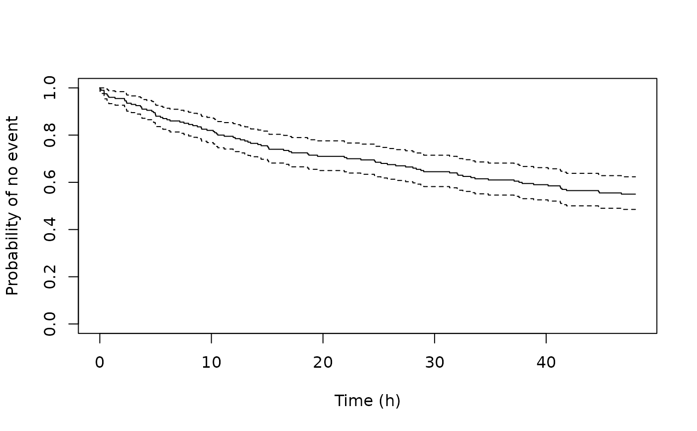
The events give a Kaplan-Meier estimate directly:
last <- tte[!duplicated(tte$id, fromLast = TRUE), ]
if (requireNamespace("survival", quietly = TRUE)) {
  fit <- survival::survfit(survival::Surv(time, sim) ~ 1, data = last)
  plot(fit, xlab = "Time (h)", ylab = "Probability of no event")
}
Options
| Option | Default | Meaning |
|---|---|---|
eventType |
"exact" |
"exact" or "intervalCensored" event
times |
maxEventNumber |
Inf |
maximum number of events (1 for one-off) |
rightCensoringTime |
last record of the endpoint | end of the observation window |
intervalLength |
tenth of the observation window | interval length for "intervalCensored"
|
dropout |
FALSE |
the event ends all observations (needs
maxEventNumber = 1) |
With eventType = "intervalCensored" the rows are the
ends of each interval, with sim = 1 when the interval holds
an event:
ic <- seizure() |>
  model(ev ~ tte(haz, eventType = "intervalCensored", intervalLength = 12,
                 maxEventNumber = 1))
s <- withr::with_seed(42, rxSolve(ic, e))
s <- as.data.frame(s)
head(s[s$CMT == 4, c("id", "time", "sim")])
#>    id time sim
#> 2   1    0   0
#> 6   1   12   1
#> 17  2    0   0
#> 21  2   12   0
#> 25  2   24   1
#> 33  3    0   0
dropout = TRUE makes the event end the subject’s
observations of every endpoint, as in a joint PK/dropout simulation:
dr <- seizure() |>
  model(ev ~ tte(haz, maxEventNumber = 1, dropout = TRUE))
s <- withr::with_seed(42, as.data.frame(rxSolve(dr, e)))
tapply(s$time[s$CMT == 3], s$id[s$CMT == 3], max)[1:10]
#>  1  2  3  4  5  6  7  8  9 10
#>  8 12  4 48  8 16 36 24 48  0
Repeated events
Without maxEventNumber the events repeat, each using the
cumulative hazard since the previous event. tteTime(ev)
(the time of the last event, or the window start) and
tteCount(ev) (the events so far) can be used in the model,
for example in a Weibull renewal hazard:
renewal <- function() {
  ini({
    te <- 5
    sh <- 2
  })
  model({
    haz <- sh / te * ((time - tteTime(ev)) / te)^(sh - 1)
    ev ~ tte(haz)
  })
}
s <- withr::with_seed(1, as.data.frame(rxSolve(renewal(), et(c(0, 50)) |> et(id = 1:100))))
table(tapply(s$sim, s$id, sum))
#>
#>  7  8  9 10 11 12 13 14 15 16
#>  2  5  8 21 26 19 12  3  3  1
tteTime() and tteCount() are part of the
model syntax, listed with the other functions in
rxSupportedFuns().
Choosing a solver
Every ODE solving method except the adjoint sensitivity
methods (rk4s, liblsodaadj, …) simulates
tte() endpoints. The root finder only asks the solver to
re-solve part of an interval from its saved start, so the event times
are found to the accuracy of whichever solver does the work, and the
random thresholds do not depend on the method:
f <- function() {
  ini({
    te <- 10
    sh <- 1.5
  })
  model({
    haz <- sh / te * (time / te)^(sh - 1)
    ev ~ tte(haz, maxEventNumber = 1)
  })
}
e <- et(c(0, 100)) |> et(id = 1:5)
sapply(c("liblsoda", "dop853", "rk4", "lsode", "cvode"), function(m) {
  s <- withr::with_seed(2, as.data.frame(rxSolve(f(), e, method = m)))
  s$time[s$sim == 1]
})
#>       liblsoda    dop853       rk4     lsode     cvode
#> [1,] 15.223412 15.223417 15.223424 15.223412 15.223384
#> [2,] 15.810482 15.810487 15.810494 15.810482 15.810452
#> [3,]  5.510067  5.510068  5.510080  5.510067  5.510062
#> [4,]  2.935511  2.935511  2.935527  2.935511  2.935505
#> [5,]  8.398936  8.398938  8.398948  8.398936  8.398917
liblsoda (the default) keeps its integrator history
between records. The other methods run in a shared record loop that
restarts the solver at each record, which costs little for the one-step
methods (Runge-Kutta, Rosenbrock) and more for the multistep ones. The
Fortran lsoda, lsode and bdf
methods solve one subject at a time. dense = TRUE falls
back to standard output.
A hazard may use delay(). The record loop then solves
each interval with a dense solver (dop853+ros4,
dop853 or ros4), whose steps record the
history delay() reads, and an event rewinds that history
with the state. Any state may be delayed, including the cumulative
hazard itself (delay(rx.tteH.ev, tau)), but a delayed
cumulative hazard cannot be combined with steady-state doses, since the
hazard has no steady state:
dde <- function() {
  ini({
    k <- 0.3
    lambda <- 0.005
    beta <- 0.02
    tau <- 2
  })
  model({
    d/dt(central) <- -k * delay(central, tau)
    haz <- lambda * exp(beta * central)
    ev ~ tte(haz, maxEventNumber = 1)
  })
}
ed <- et(amt = 100, cmt = "central") |> et(c(0, 48), cmt = "ev") |> et(id = 1:5)
s <- withr::with_seed(3, as.data.frame(rxSolve(dde(), ed)))
#> [====|====|====|====|====|====|====|====|====|====] 0:00:00
s[, c("id", "time", "sim", "central")]
#>    id      time sim       central
#> 1   1  0.000000   0  1.000000e+02
#> 2   1 48.000000   0 -2.010272e-05
#> 3   2  0.000000   0  1.000000e+02
#> 4   2 48.000000   0 -2.010272e-05
#> 5   3  0.000000   0  1.000000e+02
#> 6   3  3.330003   1  6.010032e+01
#> 7   4  0.000000   0  1.000000e+02
#> 8   4 48.000000   0 -2.010272e-05
#> 9   5  0.000000   0  1.000000e+02
#> 10  5 48.000000   0 -2.010272e-05