Chapter 11 Simulation

11.1 Single Subject solving

Originally, rxode2 was only created to solve ODEs for one individual. That is a single system without any changes in individual parameters.

Of course this is still supported, the classic examples are found in rxode2 intro.

This article discusses the differences between multiple subject and single subject solving. There are three differences:

• Single solving does not solve each ID in parallel
• Single solving lacks the id column in parameters($params) as well as in the actual dataset.
• Single solving allows parameter exploration easier because each parameter can be modified. With multiple subject solves, you have to make sure to update each individual parameter.

The first obvious difference is in speed; With multiple subjects you can run each subject ID in parallel. For more information and examples of the speed gains with multiple subject solving see the Speeding up rxode2 vignette.

The next difference is the amount of information output in the final data.

Taking the 2 compartment indirect response model originally in the tutorial:

library(rxode2)

mod1 <- function() {
  ini({
    KA=2.94E-01
    CL=1.86E+01
    V2=4.02E+01
    Q=1.05E+01
    V3=2.97E+02
    Kin=1
    Kout=1
    EC50=200
  })
  model({
    C2 = centr/V2
    C3 = peri/V3
    d/dt(depot) =-KA*depot
    d/dt(centr) = KA*depot - CL*C2 - Q*C2 + Q*C3
    d/dt(peri)  =                    Q*C2 - Q*C3
    d/dt(eff)  = Kin - Kout*(1-C2/(EC50+C2))*eff
    eff(0) = 1
  })
}
  
et <- et(amount.units='mg', time.units='hours') %>%
    et(dose=10000, addl=9, ii=12) %>%
    et(amt=20000, nbr.doses=5, start.time=120, dosing.interval=24) %>%
    et(0:240) # sampling

Now a simple solve

x <- rxSolve(mod1, et)
x

#> ── Solved rxode2 object ──
#> ── Parameters (x$params): ──
#>      KA      CL      V2       Q      V3     Kin    Kout    EC50 
#>   0.294  18.600  40.200  10.500 297.000   1.000   1.000 200.000 
#> ── Initial Conditions (x$inits): ──
#> depot centr  peri   eff 
#>     0     0     0     1 
#> ── First part of data (object): ──
#> # A tibble: 241 × 7
#>   time    C2    C3  depot centr  peri   eff
#>    [h] <dbl> <dbl>  <dbl> <dbl> <dbl> <dbl>
#> 1    0   0   0     10000     0     0   1   
#> 2    1  44.4 0.920  7453. 1784.  273.  1.08
#> 3    2  54.9 2.67   5554. 2206.  794.  1.18
#> 4    3  51.9 4.46   4140. 2087. 1324.  1.23
#> 5    4  44.5 5.98   3085. 1789. 1776.  1.23
#> 6    5  36.5 7.18   2299. 1467. 2132.  1.21
#> # ℹ 235 more rows

print(x)

#> ── Solved rxode2 object ──
#> ── Parameters ($params): ──
#>      KA      CL      V2       Q      V3     Kin    Kout    EC50 
#>   0.294  18.600  40.200  10.500 297.000   1.000   1.000 200.000 
#> ── Initial Conditions ($inits): ──
#> depot centr  peri   eff 
#>     0     0     0     1 
#> ── First part of data (object): ──
#> # A tibble: 241 × 7
#>   time    C2    C3  depot centr  peri   eff
#>    [h] <dbl> <dbl>  <dbl> <dbl> <dbl> <dbl>
#> 1    0   0   0     10000     0     0   1   
#> 2    1  44.4 0.920  7453. 1784.  273.  1.08
#> 3    2  54.9 2.67   5554. 2206.  794.  1.18
#> 4    3  51.9 4.46   4140. 2087. 1324.  1.23
#> 5    4  44.5 5.98   3085. 1789. 1776.  1.23
#> 6    5  36.5 7.18   2299. 1467. 2132.  1.21
#> # ℹ 235 more rows

plot(x, C2, eff)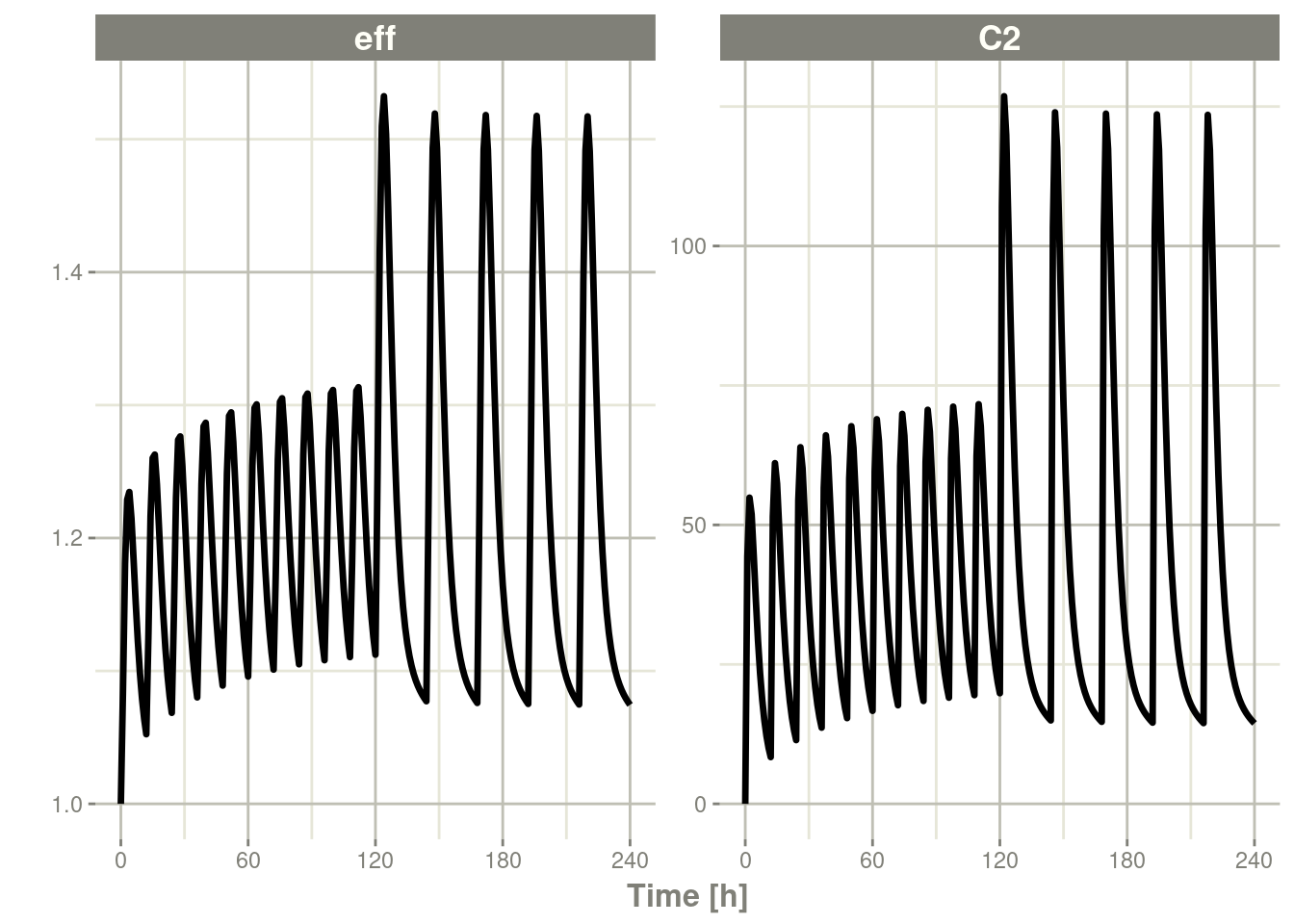

To better see the differences between the single solve, you can solve for 2 individuals

x2 <- rxSolve(mod1, et %>% et(id=1:2), params=data.frame(CL=c(18.6, 7.6)))
print(x2)

#> ── Solved rxode2 object ──
#> ── Parameters ($params): ──
#> # A tibble: 2 × 9
#>   id       KA    CL    V2     Q    V3   Kin  Kout  EC50
#>   <fct> <dbl> <dbl> <dbl> <dbl> <dbl> <dbl> <dbl> <dbl>
#> 1 1     0.294  18.6  40.2  10.5   297     1     1   200
#> 2 2     0.294   7.6  40.2  10.5   297     1     1   200
#> ── Initial Conditions ($inits): ──
#> depot centr  peri   eff 
#>     0     0     0     1 
#> ── First part of data (object): ──
#> # A tibble: 482 × 8
#>      id time    C2    C3  depot centr  peri   eff
#>   <int>  [h] <dbl> <dbl>  <dbl> <dbl> <dbl> <dbl>
#> 1     1    0   0   0     10000     0     0   1   
#> 2     1    1  44.4 0.920  7453. 1784.  273.  1.08
#> 3     1    2  54.9 2.67   5554. 2206.  794.  1.18
#> 4     1    3  51.9 4.46   4140. 2087. 1324.  1.23
#> 5     1    4  44.5 5.98   3085. 1789. 1776.  1.23
#> 6     1    5  36.5 7.18   2299. 1467. 2132.  1.21
#> # ℹ 476 more rows

plot(x2, C2, eff)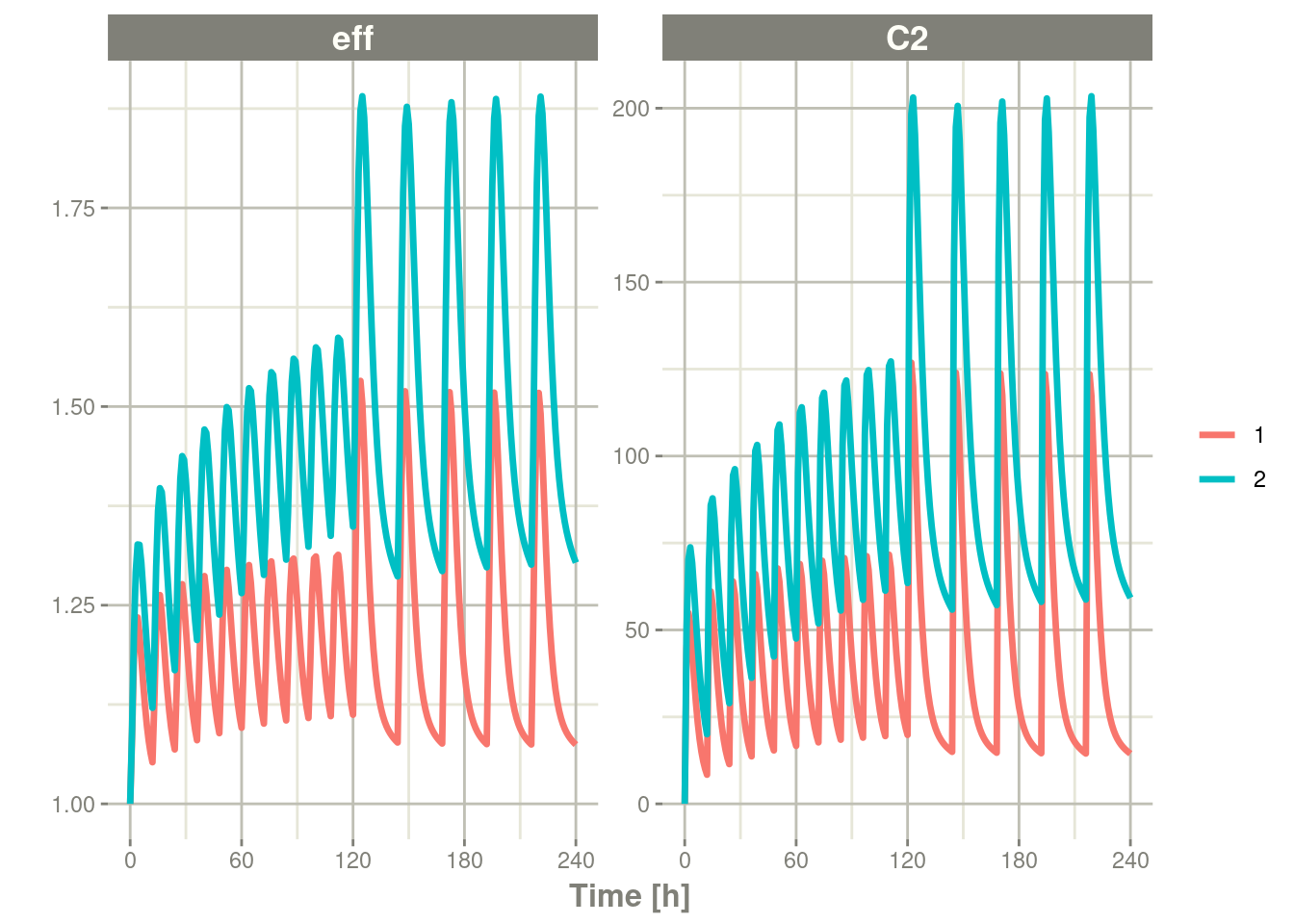

By observing the two solves, you can see:

• A multiple subject solve contains the id column both in the data frame and then data frame of parameters for each subject.

The last feature that is not as obvious, modifying the individual parameters. For single subject data, you can modify the rxode2 data frame changing initial conditions and parameter values as if they were part of the data frame, as described in the rxode2 Data Frames.

For multiple subject solving, this feature still works, but requires care when supplying each individual’s parameter value, otherwise you may change the solve and drop parameter for key individuals.

11.1.1 Summary of Single solve vs Multiple subject solving

Feature	Single Subject Solve	Multiple Subject Solve
Parallel	None	Each Subject
$params	data.frame with one parameter value	data.frame with one parameter per subject (w/ID column)
solved data	Can modify individual parameters with $ syntax	Have to modify all the parameters to update solved object

11.2 Population Simulations with rxode2

11.2.1 Simulation of Variability with rxode2

In pharmacometrics the nonlinear-mixed effect modeling software (like nlmixr) characterizes the between-subject variability. With this between subject variability you can simulate new subjects.

Assuming that you have a 2-compartment, indirect response model, you can set create an rxode2 model describing this system below:

11.2.1.1 Setting up the rxode2 model

library(rxode2)

set.seed(32)
rxSetSeed(32)

mod <- function() {
  ini({
    KA <- 2.94E-01
    TCl <- 1.86E+01
    # between subject variability
    eta.Cl ~ 0.4^2
    V2 <- 4.02E+01
    Q <- 1.05E+01
    V3 <- 2.97E+02
    Kin <- 1
    Kout <- 1
    EC50 <- 200
  })
  model({
    C2 <- centr/V2
    C3 <- peri/V3
    CL <-  TCl*exp(eta.Cl) ## This is coded as a variable in the model
    d/dt(depot) <- -KA*depot
    d/dt(centr) <- KA*depot - CL*C2 - Q*C2 + Q*C3
    d/dt(peri)  <-                    Q*C2 - Q*C3
    d/dt(eff)   <- Kin - Kout*(1-C2/(EC50+C2))*eff
    eff(0) <- 1
  })
}

11.2.1.2 Simulating

The next step to simulate is to create the dosing regimen for overall simulation:

ev <- et(amountUnits="mg", timeUnits="hours") %>%
  et(amt=10000, cmt="centr")

If you wish, you can also add sampling times (though rxode2 can fill these in for you):

ev <- ev %>% et(0,48, length.out=100)

Note the et takes similar arguments as seq when adding sampling times. There are more methods to adding sampling times and events to make complex dosing regimens (See the event vignette). This includes ways to add variability to the both the sampling and dosing times).

Once this is complete you can simulate using the rxSolve routine:

sim  <- rxSolve(mod, ev, nSub=100)

#> using C compiler: ‘gcc (Ubuntu 11.4.0-1ubuntu1~22.04) 11.4.0’

To quickly look and customize your simulation you use the default plot routine. Since this is an rxode2 object, it will create a ggplot2 object that you can modify as you wish. The extra parameter to the plot tells rxode2/R what piece of information you are interested in plotting. In this case, we are interested in looking at the derived parameter C2:

11.2.1.3 Checking the simulation with plot

library(ggplot2)
### The plots from rxode2 are ggplots so they can be modified with
### standard ggplot commands.
plot(sim, C2, log="y") +
    ylab("Central Compartment")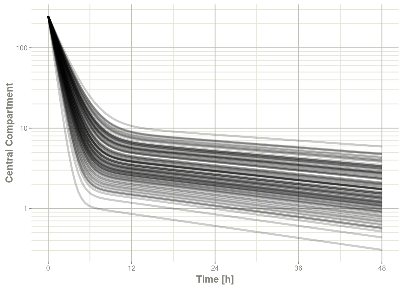 

Of course this additional parameter could also be a state value, like eff:

### They also takes many of the standard plot arguments; See ?plot
plot(sim, eff, ylab="Effect")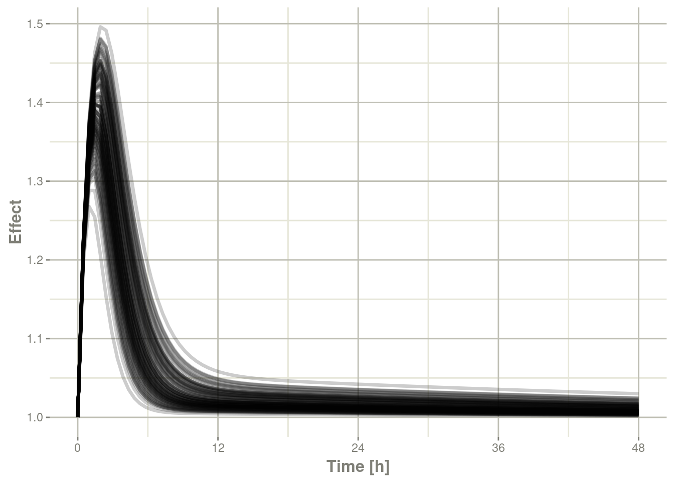

Or you could even look at the two side-by-side:

plot(sim, C2, eff)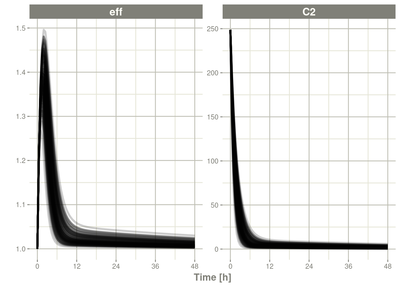

Or stack them with patchwork

library(patchwork)
plot(sim, C2, log="y") / plot(sim, eff)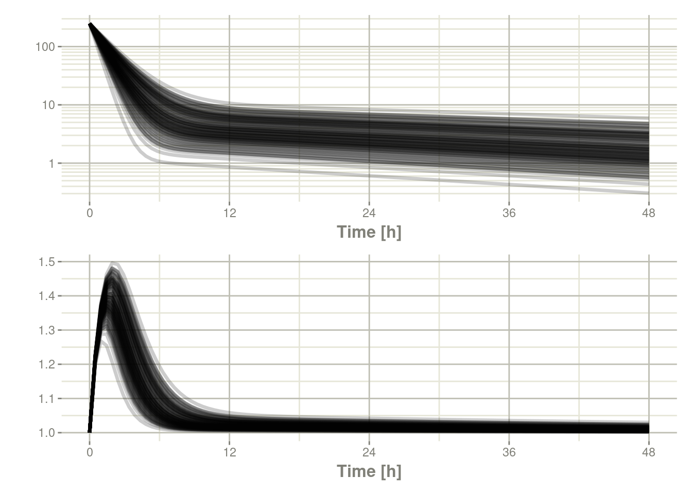

11.2.1.4 Processing the data to create summary plots

Usually in pharmacometric simulations it is not enough to simply simulate the system. We have to do something easier to digest, like look at the central and extreme tendencies of the simulation.

Since the rxode2 solve object is a type of data frame

It is now straightforward to perform calculations and generate plots with the simulated data. You can

Below, the 5th, 50th, and 95th percentiles of the simulated data are plotted.

confint(sim, "C2", level=0.95) %>%
    plot(ylab="Central Concentration", log="y")

#> ! in order to put confidence bands around the intervals, you need at least 2500 simulations

#> summarizing data...done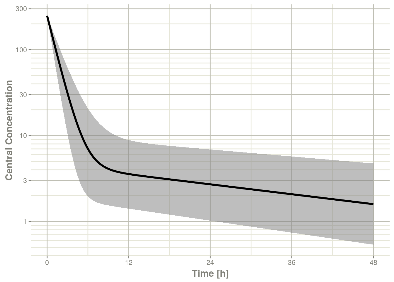

confint(sim, "eff", level=0.95) %>%
    plot(ylab="Effect")

#> ! in order to put confidence bands around the intervals, you need at least 2500 simulations

#> summarizing data...done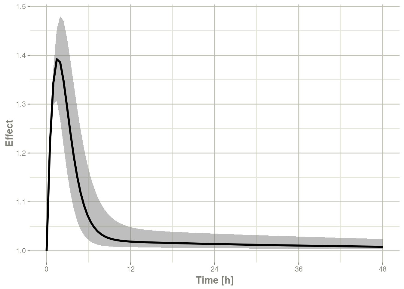

Note that you can see the parameters that were simulated for the example

head(sim$param)

#>   sim.id    KA  TCl   V2    Q  V3 Kin Kout EC50      eta.Cl
#> 1      1 0.294 18.6 40.2 10.5 297   1    1  200 -0.61812276
#> 2      2 0.294 18.6 40.2 10.5 297   1    1  200  0.08180225
#> 3      3 0.294 18.6 40.2 10.5 297   1    1  200  0.90546786
#> 4      4 0.294 18.6 40.2 10.5 297   1    1  200  0.47668266
#> 5      5 0.294 18.6 40.2 10.5 297   1    1  200  0.15939498
#> 6      6 0.294 18.6 40.2 10.5 297   1    1  200 -0.14083691

11.2.1.5 Simulation of unexplained variability (sigma)

In addition to conveniently simulating between subject variability, you can also easily simulate unexplained variability.

One way to do that is to create a rxode2 model with the endpoints defined. Model piping can do this while keeping the model intact:

mod2 <- mod %>%
  model(eff ~ add(eff.sd), append=TRUE) %>%
  model(C2 ~ prop(prop.sd), append=TRUE) %>%
  ini(eff.sd=sqrt(0.1), prop.sd=sqrt(0.1))

#> ℹ add residual parameter `eff.sd` and set estimate to 1

#> ℹ add residual parameter `prop.sd` and set estimate to 1

#> ℹ change initial estimate of `eff.sd` to `0.316227766016838`

#> ℹ change initial estimate of `prop.sd` to `0.316227766016838`

You can see how the dataset should be defined with $multipleEndpoint:

mod2$multipleEndpoint

#>   variable                cmt                dvid*
#> 1  eff ~ … cmt='eff' or cmt=4 dvid='eff' or dvid=1
#> 2   C2 ~ …  cmt='C2' or cmt=5  dvid='C2' or dvid=2

Here you see the endpoints should be defined for eff and C2:

ev <- et(amountUnits="mg", timeUnits="hours") %>%
  et(amt=10000, cmt="centr") %>%
  et(seq(0,48, length.out=100), cmt="eff") %>%
  et(seq(0,48, length.out=100), cmt="C2")

Which allows you to solve the system:

sim  <- rxSolve(mod2, ev, nSub=100)

#> using C compiler: ‘gcc (Ubuntu 11.4.0-1ubuntu1~22.04) 11.4.0’

Since this is simulated from a model with the residual specification included and a multiple endpoint model, you can summarize for each endpoint by simply taking a confidence interval of "sim":

s <- confint(sim, "sim")

#> ! in order to put confidence bands around the intervals, you need at least 2500 simulations

#> summarizing data...done

plot(s)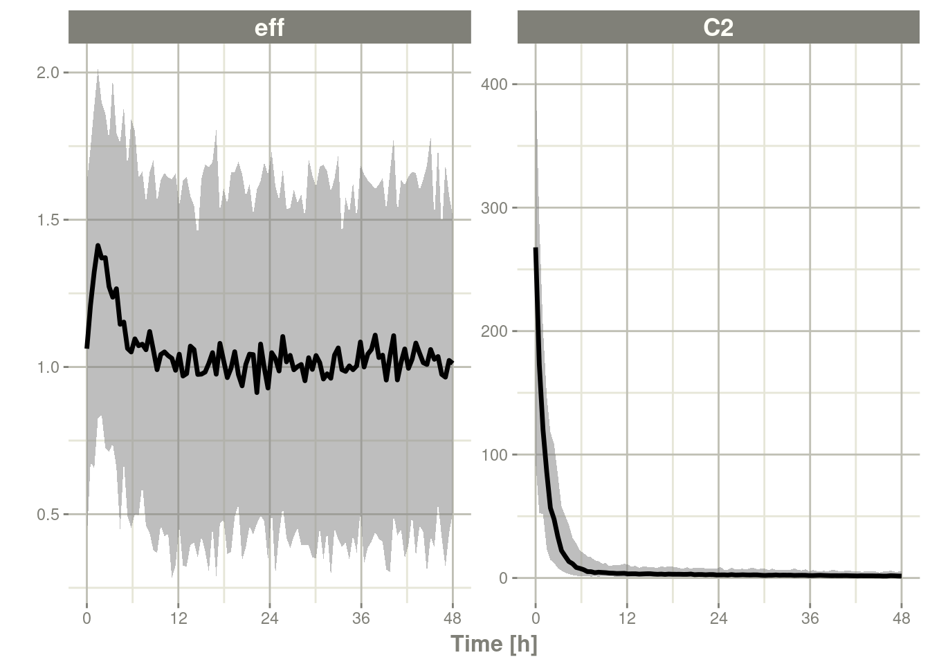

If you want to subset to a specific endpoint, like eff you can create the confidence interval for only that endpoint by using the specification sim.eff, where the endpoint name is separated from sim by a dot:

seff <- confint(sim, "sim.eff")

#> ! in order to put confidence bands around the intervals, you need at least 2500 simulations

#> summarizing data...done

plot(seff)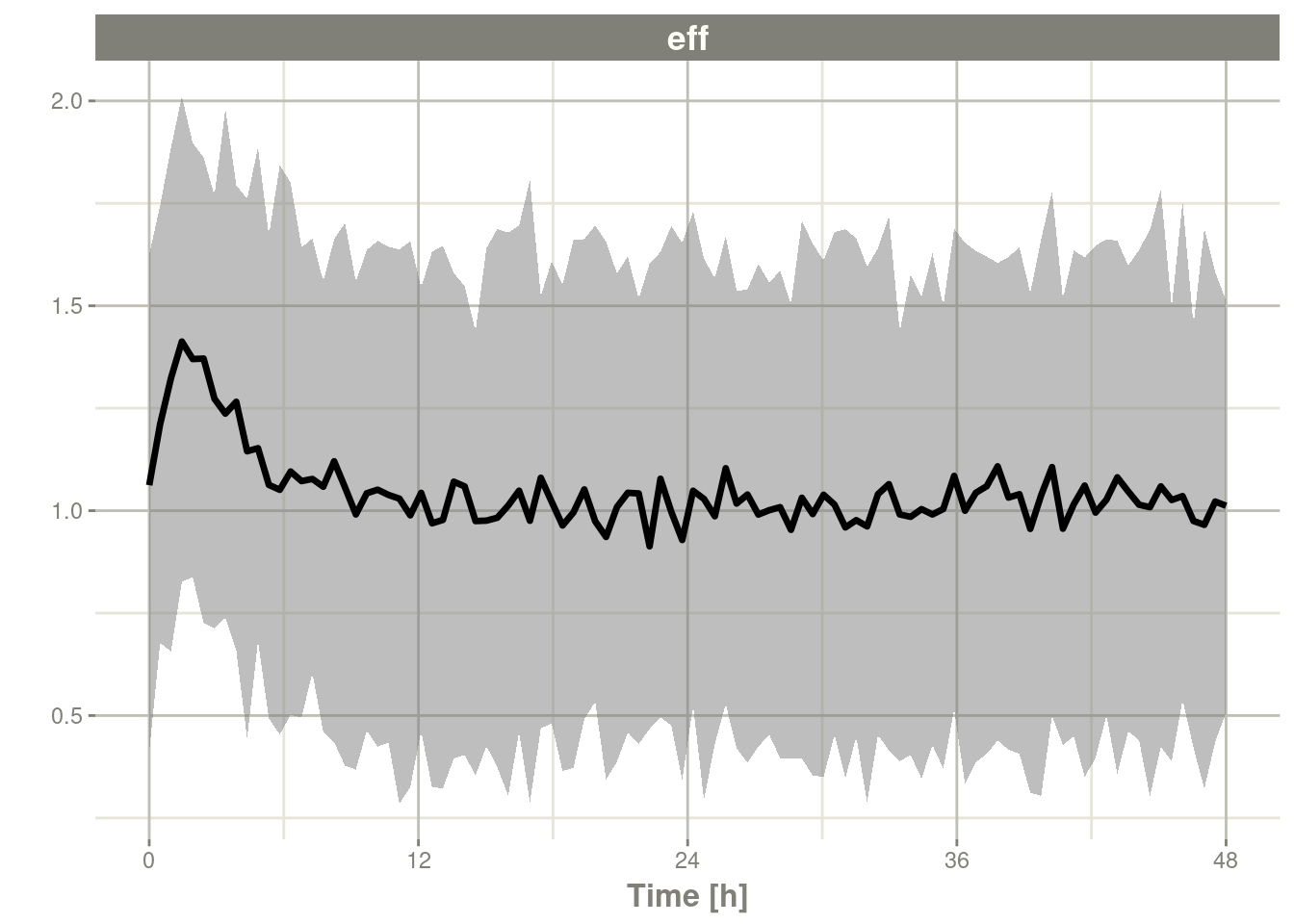

11.2.1.6 Simulation of Individuals

Sometimes you may want to match the dosing and observations of individuals in a clinical trial. To do this you will have to create a data.frame using the rxode2 event specification as well as an ID column to indicate an individual. The rxode2 event vignette talks more about how these datasets should be created.

library(dplyr)
ev1 <- et(amountUnits="mg", timeUnits="hours") %>%
    et(amt=10000, cmt=2) %>%
    et(0,48,length.out=10)

ev2 <- et(amountUnits="mg", timeUnits="hours") %>%
    et(amt=5000, cmt=2) %>%
    et(0,48,length.out=8)

dat <- rbind(data.frame(ID=1, ev1$get.EventTable()),
             data.frame(ID=2, ev2$get.EventTable()))


### Note the number of subject is not needed since it is determined by the data
sim  <- rxSolve(mod, dat)

sim %>% select(id, time, eff, C2)

#>    id          time      eff          C2
#> 1   1  0.000000 [h] 1.000000 248.7562189
#> 2   1  5.333333 [h] 1.028494   2.0252374
#> 3   1 10.666667 [h] 1.006985   1.3313641
#> 4   1 16.000000 [h] 1.005916   1.1507552
#> 5   1 21.333333 [h] 1.005117   0.9953618
#> 6   1 26.666667 [h] 1.004426   0.8609553
#> 7   1 32.000000 [h] 1.003828   0.7446975
#> 8   1 37.333333 [h] 1.003311   0.6441382
#> 9   1 42.666667 [h] 1.002864   0.5571571
#> 10  1 48.000000 [h] 1.002477   0.4819218
#> 11  2  0.000000 [h] 1.000000 124.3781095
#> 12  2  6.857143 [h] 1.025417   3.0885681
#> 13  2 13.714286 [h] 1.009566   1.8539299
#> 14  2 20.571429 [h] 1.008138   1.5920429
#> 15  2 27.428571 [h] 1.007015   1.3724957
#> 16  2 34.285714 [h] 1.006048   1.1832665
#> 17  2 41.142857 [h] 1.005214   1.0201272
#> 18  2 48.000000 [h] 1.004495   0.8794807

11.3 Simulation of Clinical Trials

By either using a simple single event table, or data from a clinical trial as described above, a complete clinical trial simulation can be performed.

Typically in clinical trial simulations you want to account for the uncertainty in the fixed parameter estimates, and even the uncertainty in both your between subject variability as well as the unexplained variability.

rxode2 allows you to account for these uncertainties by simulating multiple virtual “studies,” specified by the parameter nStud. Each of these studies samples a realization of fixed effect parameters and covariance matrices for the between subject variability(omega) and unexplained variabilities (sigma). Depending on the information you have from the models, there are a few strategies for simulating a realization of the omega and sigma matrices.

The first strategy occurs when either there is not any standard errors for standard deviations (or related parameters), or there is a modeled correlation in the model you are simulating from. In that case the suggested strategy is to use the inverse Wishart (parameterized to scale to the conjugate prior)/scaled inverse chi distribution. this approach uses a single parameter to inform the variability of the covariance matrix sampled (the degrees of freedom).

The second strategy occurs if you have standard errors on the variance/standard deviation with no modeled correlations in the covariance matrix. In this approach you perform separate simulations for the standard deviations and the correlation matrix. First you simulate the variance/standard deviation components in the thetaMat multivariate normal simulation. After simulation and transformation to standard deviations, a correlation matrix is simulated using the degrees of freedom of your covariance matrix. Combining the simulated standard deviation with the simulated correlation matrix will give a simulated covariance matrix. For smaller dimension covariance matrices (dimension < 10x10) it is recommended you use the lkj distribution to simulate the correlation matrix. For higher dimension covariance matrices it is suggested you use the inverse wishart distribution (transformed to a correlation matrix) for the simulations.

The covariance/variance prior is simulated from rxode2s cvPost() function.

11.3.1 Simulation from inverse Wishart correlations

An example of this simulation is below:

### Creating covariance matrix
tmp <- matrix(rnorm(8^2), 8, 8)
tMat <- tcrossprod(tmp, tmp) / (8 ^ 2)
dimnames(tMat) <- list(NULL, names(mod2$theta)[1:8])

sim  <- rxSolve(mod2, ev, nSub=100, thetaMat=tMat, nStud=10,
                dfSub=10, dfObs=100)

s <-sim %>% confint("sim")

#> summarizing data...done

plot(s)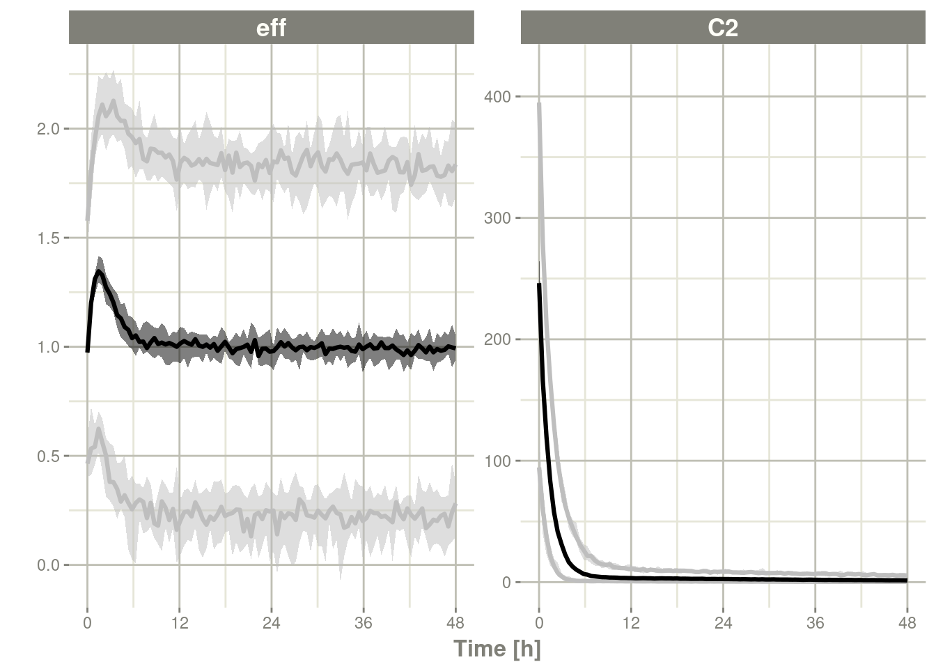

If you wish you can see what omega and sigma was used for each virtual study by accessing them in the solved data object with $omega.list and $sigma.list:

head(sim$omegaList)

#> [[1]]
#>           eta.Cl
#> eta.Cl 0.1676778
#> 
#> [[2]]
#>           eta.Cl
#> eta.Cl 0.2917085
#> 
#> [[3]]
#>           eta.Cl
#> eta.Cl 0.1776813
#> 
#> [[4]]
#>           eta.Cl
#> eta.Cl 0.1578682
#> 
#> [[5]]
#>           eta.Cl
#> eta.Cl 0.1845614
#> 
#> [[6]]
#>           eta.Cl
#> eta.Cl 0.3282268

head(sim$sigmaList)

#> [[1]]
#>            rxerr.eff   rxerr.C2
#> rxerr.eff 1.12416983 0.04197039
#> rxerr.C2  0.04197039 0.97293971
#> 
#> [[2]]
#>             rxerr.eff    rxerr.C2
#> rxerr.eff  0.84311199 -0.06277998
#> rxerr.C2  -0.06277998  1.22140938
#> 
#> [[3]]
#>           rxerr.eff  rxerr.C2
#> rxerr.eff 0.9834771 0.1060251
#> rxerr.C2  0.1060251 1.0024751
#> 
#> [[4]]
#>            rxerr.eff   rxerr.C2
#> rxerr.eff 1.25556975 0.07690868
#> rxerr.C2  0.07690868 0.90991261
#> 
#> [[5]]
#>           rxerr.eff  rxerr.C2
#> rxerr.eff  1.116261 -0.184748
#> rxerr.C2  -0.184748  1.320288
#> 
#> [[6]]
#>            rxerr.eff   rxerr.C2
#> rxerr.eff 0.93539238 0.07270049
#> rxerr.C2  0.07270049 0.98648424

You can also see the parameter realizations from the $params data frame.

11.3.2 Simulate using variance/standard deviation standard errors

Lets assume we wish to simulate from the nonmem run included in xpose

First we setup the model; Since we are taking this from nonmem and would like to use the more free-form style from the classic rxode2 model we start from the classic model:

rx1 <- rxode2({
  cl <- tcl*(1+crcl.cl*(CLCR-65)) * exp(eta.cl)
  v <- tv * WT * exp(eta.v)
  ka <- tka * exp(eta.ka)
  ipred <- linCmt()
  obs <- ipred * (1 + prop.sd) + add.sd 
})

#> using C compiler: ‘gcc (Ubuntu 11.4.0-1ubuntu1~22.04) 11.4.0’

Next we input the estimated parameters:

theta <- c(tcl=2.63E+01, tv=1.35E+00, tka=4.20E+00, tlag=2.08E-01,
           prop.sd=2.05E-01, add.sd=1.06E-02, crcl.cl=7.17E-03,
           ## Note that since we are using the separation strategy the ETA variances are here too
           eta.cl=7.30E-02,  eta.v=3.80E-02, eta.ka=1.91E+00)

And also their covariances; To me, the easiest way to create a named covariance matrix is to use lotri():

thetaMat <- lotri(
    tcl + tv + tka + tlag + prop.sd + add.sd + crcl.cl + eta.cl + eta.v + eta.ka ~
        c(7.95E-01,
          2.05E-02, 1.92E-03,
          7.22E-02, -8.30E-03, 6.55E-01,
          -3.45E-03, -6.42E-05, 3.22E-03, 2.47E-04,
          8.71E-04, 2.53E-04, -4.71E-03, -5.79E-05, 5.04E-04,
          6.30E-04, -3.17E-06, -6.52E-04, -1.53E-05, -3.14E-05, 1.34E-05,
          -3.30E-04, 5.46E-06, -3.15E-04, 2.46E-06, 3.15E-06, -1.58E-06, 2.88E-06,
          -1.29E-03, -7.97E-05, 1.68E-03, -2.75E-05, -8.26E-05, 1.13E-05, -1.66E-06, 1.58E-04,
          -1.23E-03, -1.27E-05, -1.33E-03, -1.47E-05, -1.03E-04, 1.02E-05, 1.67E-06, 6.68E-05, 1.56E-04,
          7.69E-02, -7.23E-03, 3.74E-01, 1.79E-03, -2.85E-03, 1.18E-05, -2.54E-04, 1.61E-03, -9.03E-04, 3.12E-01))

evw <- et(amount.units="mg", time.units="hours") %>%
    et(amt=100) %>%
    ## For this problem we will simulate with sampling windows
    et(list(c(0, 0.5),
       c(0.5, 1),
       c(1, 3),
       c(3, 6),
       c(6, 12))) %>%
    et(id=1:1000)

### From the run we know that:
###   total number of observations is: 476
###    Total number of individuals:     74
sim  <- rxSolve(rx1, theta, evw,  nSub=100, nStud=10,
                thetaMat=thetaMat,
                ## Match boundaries of problem
                thetaLower=0, 
                sigma=c("prop.sd", "add.sd"), ## Sigmas are standard deviations
                sigmaXform="identity", # default sigma xform="identity"
                omega=c("eta.cl", "eta.v", "eta.ka"), ## etas are variances
                omegaXform="variance", # default omega xform="variance"
                iCov=data.frame(WT=rnorm(1000, 70, 15), CLCR=rnorm(1000, 65, 25)),
                dfSub=74, dfObs=476);

#> ℹ thetaMat has too many items, ignored: 'tlag'

print(sim)

#> ── Solved rxode2 object ──
#> ── Parameters ($params): ──
#> # A tibble: 10,000 × 9
#>    sim.id id      tcl crcl.cl eta.cl    tv   eta.v   tka   eta.ka
#>     <int> <fct> <dbl>   <dbl>  <dbl> <dbl>   <dbl> <dbl>    <dbl>
#>  1      1 1      28.5    1.07 -0.209  1.64  0.572   4.45 -0.681  
#>  2      1 2      28.5    1.07 -1.26   1.64 -0.517   4.45 -0.0415 
#>  3      1 3      28.5    1.07  0.241  1.64  0.0818  4.45  1.23   
#>  4      1 4      28.5    1.07  0.150  1.64 -1.70    4.45  0.196  
#>  5      1 5      28.5    1.07  0.170  1.64  0.713   4.45 -0.502  
#>  6      1 6      28.5    1.07  1.01   1.64 -0.185   4.45 -0.00501
#>  7      1 7      28.5    1.07 -0.700  1.64 -0.0111  4.45  0.0739 
#>  8      1 8      28.5    1.07  1.49   1.64  0.438   4.45  0.640  
#>  9      1 9      28.5    1.07  0.381  1.64 -1.15    4.45  0.575  
#> 10      1 10     28.5    1.07 -0.142  1.64  0.797   4.45  0.0448 
#> # ℹ 9,990 more rows
#> ── Initial Conditions ($inits): ──
#> named numeric(0)
#> 
#> Simulation with uncertainty in:
#> • parameters ($thetaMat for changes)
#> • omega matrix ($omegaList)
#> • sigma matrix ($sigmaList)
#> 
#> ── First part of data (object): ──
#> # A tibble: 50,000 × 10
#>   sim.id    id   time    cl     v    ka   ipred     obs    WT  CLCR
#>    <int> <int>    [h] <dbl> <dbl> <dbl>   <dbl>   <dbl> <dbl> <dbl>
#> 1      1     1 0.0155  128. 181.   2.25 0.0188   0.529   62.2  69.3
#> 2      1     1 0.749   128. 181.   2.25 0.325    1.09    62.2  69.3
#> 3      1     1 1.02    128. 181.   2.25 0.310    0.908   62.2  69.3
#> 4      1     1 3.41    128. 181.   2.25 0.0721  -0.769   62.2  69.3
#> 5      1     1 7.81    128. 181.   2.25 0.00323  0.0646  62.2  69.3
#> 6      1     2 0.0833  357.  35.0  4.27 0.562    1.19    35.7 105. 
#> # ℹ 49,994 more rows

### Notice that the simulation time-points change for the individual

### If you want the same sampling time-points you can do that as well:
evw <- et(amount.units="mg", time.units="hours") %>%
    et(amt=100) %>%
    et(0, 24, length.out=50) %>%
    et(id=1:100)

sim  <- rxSolve(rx1, theta, evw,  nSub=100, nStud=10,
                thetaMat=thetaMat,
                ## Match boundaries of problem
                thetaLower=0, 
                sigma=c("prop.sd", "add.sd"), ## Sigmas are standard deviations
                sigmaXform="identity", # default sigma xform="identity"
                omega=c("eta.cl", "eta.v", "eta.ka"), ## etas are variances
                omegaXform="variance", # default omega xform="variance"
                iCov=data.frame(WT=rnorm(100, 70, 15), CLCR=rnorm(100, 65, 25)),
                dfSub=74, dfObs=476,
                resample=TRUE)

#> ℹ thetaMat has too many items, ignored: 'tlag'

s <-sim %>% confint(c("ipred"))

#> summarizing data...

#> done

plot(s)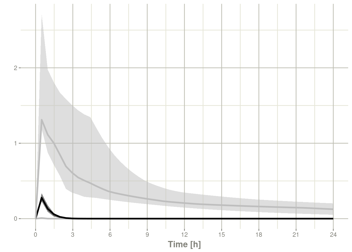

11.3.3 Simulate without uncertainty in omega or sigma parameters

If you do not wish to sample from the prior distributions of either the omega or sigma matrices, you can turn off this feature by specifying the simVariability = FALSE option when solving:

sim  <- rxSolve(mod2, ev, nSub=100, thetaMat=tMat, nStud=10,
                simVariability=FALSE)

s <-sim %>% confint(c("centr", "eff"))

#> summarizing data...done

plot(s)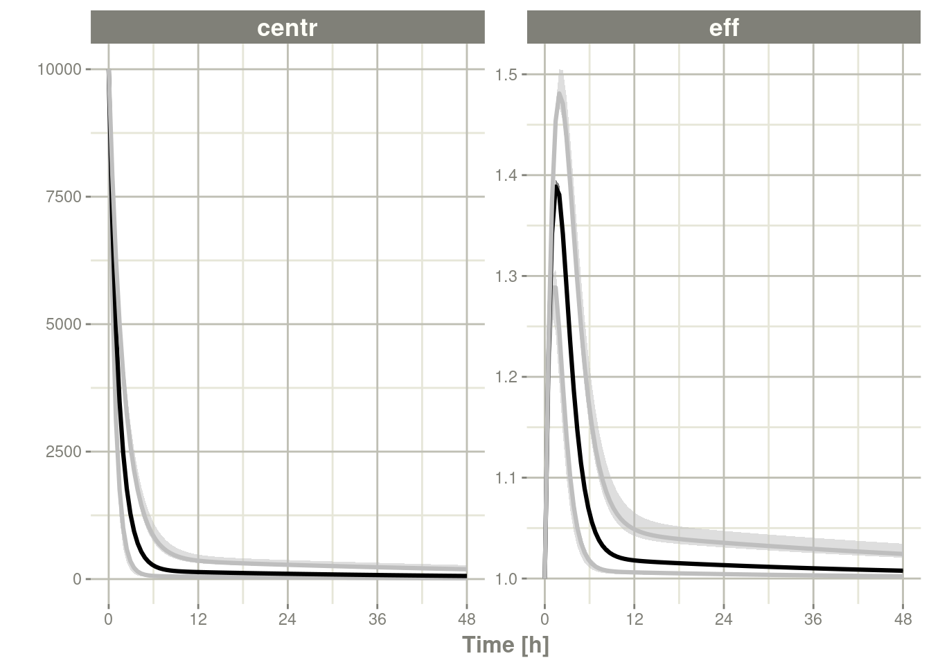

Note since realizations of omega and sigma were not simulated, $omegaList and $sigmaList both return NULL.

11.4 Using prior data for solving

rxode2 can use a single subject or multiple subjects with a single event table to solve ODEs. Additionally, rxode2 can use an arbitrary data frame with individualized events. For example when using nlmixr, you could use the theo_sd data frame

library(rxode2)
library(nlmixr2data)

### Load data from nlmixr
d <- theo_sd

### Create rxode2 model
theo <- function() {
  ini({
    tka <- 0.45 # Log Ka
    tcl <- 1 # Log Cl
    tv <- 3.45    # Log V
    eta.ka ~ 0.6
    eta.cl ~ 0.3
    eta.v ~ 0.1
  })
  model({
    ka <- exp(tka + eta.ka)
    cl <- exp(tcl + eta.cl)
    v <- exp(tv + eta.v)
    d/dt(depot) = -ka * depot
    d/dt(center) = ka * depot - cl / v * center
    cp = center / v
  }) 
}

### Create parameter dataset
library(dplyr)
parsDf <- tribble(
  ~ eta.ka, ~ eta.cl, ~ eta.v, 
  0.105, -0.487, -0.080,
  0.221, 0.144, 0.021,
  0.368, 0.031, 0.058,
 -0.277, -0.015, -0.007,
 -0.046, -0.155, -0.142,
 -0.382, 0.367, 0.203,
 -0.791, 0.160, 0.047,
 -0.181, 0.168, 0.096,
  1.420, 0.042, 0.012,
 -0.738, -0.391, -0.170,
  0.790, 0.281, 0.146,
 -0.527, -0.126, -0.198) %>%
    mutate(tka = 0.451, tcl = 1.017, tv = 3.449)

### Now solve the dataset
solveData <- rxSolve(theo, parsDf, d)

#> ℹ parameter labels from comments will be replaced by 'label()'

#> using C compiler: ‘gcc (Ubuntu 11.4.0-1ubuntu1~22.04) 11.4.0’

plot(solveData, cp)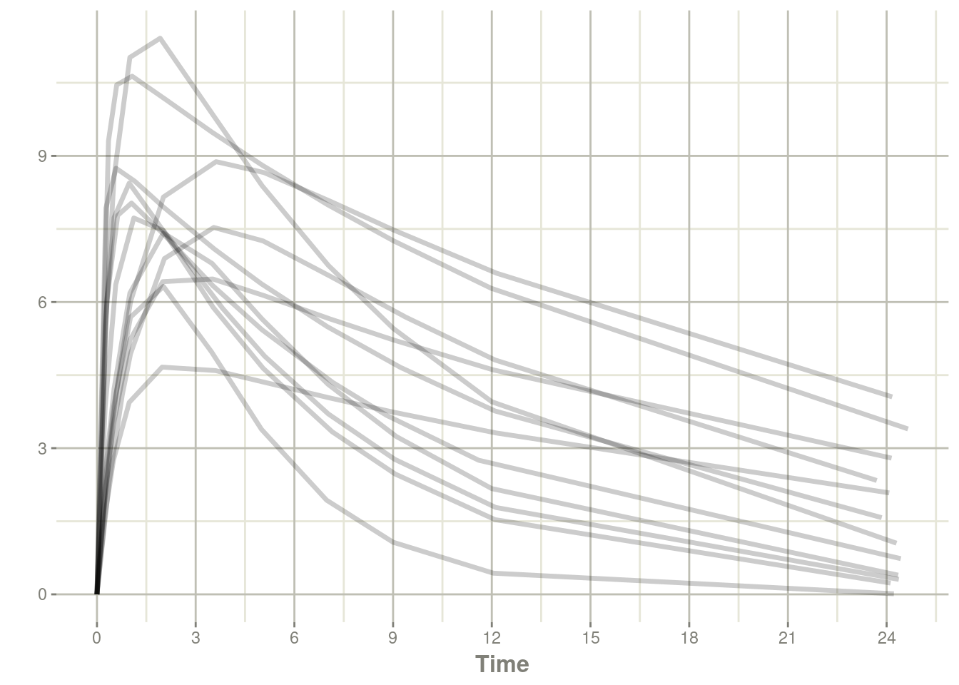

print(solveData)

#> ── Solved rxode2 object ──
#> ── Parameters ($params): ──
#> # A tibble: 12 × 7
#>    id      tka   tcl    tv  eta.ka  eta.cl   eta.v
#>    <fct> <dbl> <dbl> <dbl>   <dbl>   <dbl>   <dbl>
#>  1 1     0.451  1.02  3.45  0.309   0.561   0.0703
#>  2 2     0.451  1.02  3.45  0.251  -0.0937 -0.298 
#>  3 3     0.451  1.02  3.45 -0.564  -0.789  -0.0133
#>  4 4     0.451  1.02  3.45  1.22   -0.684  -0.0915
#>  5 5     0.451  1.02  3.45 -0.342   0.471   0.0190
#>  6 6     0.451  1.02  3.45  1.60   -0.0631  0.106 
#>  7 7     0.451  1.02  3.45 -0.476   1.16   -0.0539
#>  8 8     0.451  1.02  3.45  0.782   0.617   0.0361
#>  9 9     0.451  1.02  3.45  0.921   0.119  -0.0417
#> 10 10    0.451  1.02  3.45 -0.710  -0.265   0.0798
#> 11 11    0.451  1.02  3.45 -0.0164 -0.141   0.675 
#> 12 12    0.451  1.02  3.45 -0.183  -0.427   0.329 
#> ── Initial Conditions ($inits): ──
#>  depot center 
#>      0      0 
#> ── First part of data (object): ──
#> # A tibble: 132 × 8
#>      id  time    ka    cl     v    cp    depot center
#>   <int> <dbl> <dbl> <dbl> <dbl> <dbl>    <dbl>  <dbl>
#> 1     1  0     2.14  4.85  33.8  0    320.         0 
#> 2     1  0.25  2.14  4.85  33.8  3.85 188.       130.
#> 3     1  0.57  2.14  4.85  33.8  6.36  94.6      215.
#> 4     1  1.12  2.14  4.85  33.8  7.72  29.2      261.
#> 5     1  2.02  2.14  4.85  33.8  7.47   4.26     252.
#> 6     1  3.82  2.14  4.85  33.8  5.87   0.0909   198.
#> # ℹ 126 more rows

### Of course the fasest way to solve if you don't care about the rxode2 extra parameters is

solveData <- rxSolve(theo, parsDf, d, returnType="data.frame")

#> ℹ parameter labels from comments will be replaced by 'label()'

### solved data
dplyr::as_tibble(solveData)

#> # A tibble: 132 × 8
#>       id  time    ka    cl     v    cp    depot center
#>    <int> <dbl> <dbl> <dbl> <dbl> <dbl>    <dbl>  <dbl>
#>  1     1  0     2.19  3.49  30.2  0    3.20e+ 2    0  
#>  2     1  0.25  2.19  3.49  30.2  4.41 1.85e+ 2  133. 
#>  3     1  0.57  2.19  3.49  30.2  7.28 9.18e+ 1  219. 
#>  4     1  1.12  2.19  3.49  30.2  8.88 2.75e+ 1  268. 
#>  5     1  2.02  2.19  3.49  30.2  8.73 3.82e+ 0  263. 
#>  6     1  3.82  2.19  3.49  30.2  7.20 7.40e- 2  217. 
#>  7     1  5.1   2.19  3.49  30.2  6.21 4.48e- 3  187. 
#>  8     1  7.03  2.19  3.49  30.2  4.97 6.52e- 5  150. 
#>  9     1  9.05  2.19  3.49  30.2  3.93 7.78e- 7  119. 
#> 10     1 12.1   2.19  3.49  30.2  2.76 6.91e-10   83.2
#> # ℹ 122 more rows

data.table::data.table(solveData)

#>      id  time       ka       cl        v        cp         depot     center
#>   1:  1  0.00 2.191528 3.487816 30.15612 0.0000000  3.199920e+02   0.000000
#>   2:  1  0.25 2.191528 3.487816 30.15612 4.4061936  1.850108e+02 132.873716
#>   3:  1  0.57 2.191528 3.487816 30.15612 7.2754861  9.175521e+01 219.400454
#>   4:  1  1.12 2.191528 3.487816 30.15612 8.8789725  2.748894e+01 267.755389
#>   5:  1  2.02 2.191528 3.487816 30.15612 8.7345323  3.824416e+00 263.399632
#>  ---                                                                       
#> 128: 12  5.07 2.515775 4.435929 27.84752 5.4815780  9.259920e-04 152.648334
#> 129: 12  7.07 2.515775 4.435929 27.84752 3.9860963  6.045546e-06 111.002882
#> 130: 12  9.03 2.515775 4.435929 27.84752 2.9171213  4.369604e-08  81.234584
#> 131: 12 12.05 2.515775 4.435929 27.84752 1.8031415  4.791674e-09  50.213013
#> 132: 12 24.15 2.515775 4.435929 27.84752 0.2623903 -2.694005e-10   7.306919