Chapter 12 Examples

This section is for example models to get you started in common simulation scenarios.

12.1 Prediction only models

Prediction only models are simple to create. You use the rxode2 syntax without any ODE systems in them. A very simple example is a one-compartment model.

library(rxode2)

mod <- function(){
  model({
    ipre <- 10 * exp(-ke * t)
  })
}

Solving the rxode2 models are the same as saving the simple ODE system, but faster of course.

et  <- et(seq(0,24,length.out=50))
cmt1 <- rxSolve(mod,et,params=c(ke=0.5))

#> using C compiler: ‘gcc (Ubuntu 11.4.0-1ubuntu1~22.04) 11.4.0’

cmt1

#> ── Solved rxode2 object ──
#> ── Parameters (x$params): ──
#>  ke 
#> 0.5 
#> ── Initial Conditions (x$inits): ──
#> named numeric(0)
#> ── First part of data (object): ──
#> # A tibble: 50 × 2
#>    time  ipre
#>   <dbl> <dbl>
#> 1 0     10   
#> 2 0.490  7.83
#> 3 0.980  6.13
#> 4 1.47   4.80
#> 5 1.96   3.75
#> 6 2.45   2.94
#> # ℹ 44 more rows

12.2 Solved compartment models

Solved models are also simple to create. You simply place the linCmt() psuedo-function into your code. The linCmt() function figures out the type of model to use based on the parameter names specified.

Most often, pharmacometric models are parameterized in terms of volume and clearances. Clearances are specified by NONMEM-style names of CL, Q, Q1, Q2, etc. or distributional clearances CLD, CLD2. Volumes are specified by Central (VC or V), Peripheral/Tissue (VP, VT). While more translations are available, some example translations are below:

Another popular parameterization is in terms of micro-constants. rxode2 assumes compartment 1 is the central compartment. The elimination constant would be specified by K, Ke or Kel. Some example translations are below:

The last parameterization possible is using alpha and V and/or A/B/C. Some example translations are below:

Once the linCmt() sleuthing is complete, the 1, 2 or 3 compartment model solution is used as the value of linCmt().

The compartments where you can dose in a linear solved system are depot and central when there is an linear absorption constant in the model ka. Without any additional ODEs, these compartments are numbered depot=1 and central=2.

When the absorption constant ka is missing, you may only dose to the central compartment. Without any additional ODEs the compartment number is central=1.

These compartments take the same sort of events that a ODE model can take, and are discussed in the rxode2 events vignette.

mod <- function() {
  ini({
    kel <- 0.5
    V <- 1
  })
  model({
    ipre <- linCmt(V, kel)
  })
}

This then acts as an ODE model; You specify a dose to the depot compartment and then solve the system:

et  <- et(amt=10,time=0,cmt=depot) %>%
  et(seq(0,24,length.out=50))
cmt1 <- rxSolve(mod,et)

#> using C compiler: ‘gcc (Ubuntu 11.4.0-1ubuntu1~22.04) 11.4.0’

cmt1

#> ── Solved rxode2 object ──
#> ── Parameters (x$params): ──
#> kel   V 
#> 0.5 1.0 
#> ── Initial Conditions (x$inits): ──
#> named numeric(0)
#> ── First part of data (object): ──
#> # A tibble: 50 × 2
#>    time  ipre
#>   <dbl> <dbl>
#> 1 0     10   
#> 2 0.490  7.83
#> 3 0.980  6.13
#> 4 1.47   4.80
#> 5 1.96   3.75
#> 6 2.45   2.94
#> # ℹ 44 more rows

12.3 Mixing Solved Systems and ODEs

In addition to pure ODEs, you may mix solved systems and ODEs. The prior 2-compartment indirect response model can be simplified with a linCmt() function:

library(rxode2)
## Setup example model
mod1 <-function() {
  model({
    C2 = centr/V2
    C3 = peri/V3
    d/dt(depot) =-KA*depot
    d/dt(centr) = KA*depot - CL*C2 - Q*C2 + Q*C3
    d/dt(peri)  =                    Q*C2 - Q*C3
    d/dt(eff)  = Kin - Kout*(1-C2/(EC50+C2))*eff
  })
}

## Seup parameters and initial conditions

theta <-
    c(KA=2.94E-01, CL=1.86E+01, V2=4.02E+01, # central
      Q=1.05E+01,  V3=2.97E+02,              # peripheral
      Kin=1, Kout=1, EC50=200)               # effects

inits <- c(eff=1)

## Setup dosing event information
ev <- et(amountUnits="mg", timeUnits="hours") %>%
    et(amt=10000, addl=9, ii=12) %>%
    et(amt=20000, addl=4, time=120, ii=24) %>%
    add.sampling(0:240)

## Setup a mixed solved/ode system:
mod2 <- function() {
  model({
    ## the order of variables do not matter, the type of compartmental
    ## model is determined by the parameters specified.
    C2   = linCmt(KA, CL, V2, Q, V3);
    eff(0) = 1  ## This specifies that the effect compartment starts at 1.
    d/dt(eff) =  Kin - Kout*(1-C2/(EC50+C2))*eff;
  })
}

This allows the indirect response model above to assign the 2-compartment model to the C2 variable and the used in the indirect response model.

When mixing the solved systems and the ODEs, the solved system’s compartment is always the last compartment. This is because the solved system technically isn’t a compartment to be solved. Adding the dosing compartment to the end will not interfere with the actual ODE to be solved.

Therefore,in the two-compartment indirect response model, the effect compartment is compartment #1 while the PK dosing compartment for the depot is compartment #2.

This compartment model requires a new event table since the compartment number changed:

ev <- et(amountUnits='mg', timeUnits='hours') %>%
  et(amt=10000, addl=9, ii=12, cmt=2) %>%
  et(amt=20000, addl=4, time=120, ii=24, cmt=2) %>%
  et(0:240)

This can be solved with the following command:

x <- mod2 %>%  solve(theta, ev)

#> using C compiler: ‘gcc (Ubuntu 11.4.0-1ubuntu1~22.04) 11.4.0’

print(x)

#> ── Solved rxode2 object ──
#> ── Parameters ($params): ──
#>      KA      CL      V2       Q      V3     Kin    Kout    EC50 
#>   0.294  18.600  40.200  10.500 297.000   1.000   1.000 200.000 
#> ── Initial Conditions ($inits): ──
#> eff 
#>   1 
#> ── First part of data (object): ──
#> # A tibble: 241 × 3
#>   time    C2   eff
#>    [h] <dbl> <dbl>
#> 1    0 249.   1   
#> 2    1 121.   1.35
#> 3    2  60.3  1.38
#> 4    3  31.0  1.28
#> 5    4  17.0  1.18
#> 6    5  10.2  1.11
#> # ℹ 235 more rows

Note this solving did not require specifying the effect compartment initial condition to be 1. Rather, this is already pre-specified by eff(0)=1.

This can be solved for different initial conditions easily:

x <- mod2 %>%  solve(theta, ev,c(eff=2))
print(x)

#> ── Solved rxode2 object ──
#> ── Parameters ($params): ──
#>      KA      CL      V2       Q      V3     Kin    Kout    EC50 
#>   0.294  18.600  40.200  10.500 297.000   1.000   1.000 200.000 
#> ── Initial Conditions ($inits): ──
#> eff 
#>   2 
#> ── First part of data (object): ──
#> # A tibble: 241 × 3
#>   time    C2   eff
#>    [h] <dbl> <dbl>
#> 1    0 249.   2   
#> 2    1 121.   1.93
#> 3    2  60.3  1.67
#> 4    3  31.0  1.41
#> 5    4  17.0  1.23
#> 6    5  10.2  1.13
#> # ℹ 235 more rows

The rxode2 detective also does not require you to specify the variables in the linCmt() function if they are already defined in the block. Therefore, the following function will also work to solve the same system.

mod3 <- function() {
  ini({
    KA <- 2.94E-01
    CL <- 1.86E+01
    V2 <- 4.02E+01
    Q <- 1.05E+01
    V3 <- 2.97E+02
    Kin <- 1
    Kout <- 1
    EC50 <- 200
  })
  model({
    # Since the parameters are in the ini block, put them in linCmt so
    # that the model is detected correctly
    C2   <- linCmt(KA, CL, V2, Q, V3)
    eff(0) <- 1  ## This specifies that the effect compartment starts at 1.
    d/dt(eff) <-  Kin - Kout*(1-C2/(EC50+C2))*eff;
  })
}

x <- mod3 %>%  solve(ev)

print(x)

#> ── Solved rxode2 object ──
#> ── Parameters ($params): ──
#>      KA      CL      V2       Q      V3     Kin    Kout    EC50 
#>   0.294  18.600  40.200  10.500 297.000   1.000   1.000 200.000 
#> ── Initial Conditions ($inits): ──
#> eff 
#>   1 
#> ── First part of data (object): ──
#> # A tibble: 241 × 3
#>   time    C2   eff
#>    [h] <dbl> <dbl>
#> 1    0 249.   1   
#> 2    1 121.   1.35
#> 3    2  60.3  1.38
#> 4    3  31.0  1.28
#> 5    4  17.0  1.18
#> 6    5  10.2  1.11
#> # ℹ 235 more rows

Note that you do not specify the parameters when solving the system since they are built into the model, but you can override the parameters:

x <- mod3 %>%  solve(c(KA=10),ev)
print(x)

#> ── Solved rxode2 object ──
#> ── Parameters ($params): ──
#>    KA    CL    V2     Q    V3   Kin  Kout  EC50 
#>  10.0  18.6  40.2  10.5 297.0   1.0   1.0 200.0 
#> ── Initial Conditions ($inits): ──
#> eff 
#>   1 
#> ── First part of data (object): ──
#> # A tibble: 241 × 3
#>   time    C2   eff
#>    [h] <dbl> <dbl>
#> 1    0 249.   1   
#> 2    1 121.   1.35
#> 3    2  60.3  1.38
#> 4    3  31.0  1.28
#> 5    4  17.0  1.18
#> 6    5  10.2  1.11
#> # ℹ 235 more rows

12.4 Weight based dosing

This is an example model for weight based dosing of daptomycin. Daptomycin is a cyclic lipopeptide antibiotic from fermented Streptomyces roseosporus.

There are 3 stages for weight-based dosing simulations: - Create rxode2 model - Simulate Covariates - Create event table with weight-based dosing (merged back to covariates)

12.4.1 Creating a 2-compartment model in rxode2

library(rxode2)

## Note the time covariate is not included in the simulation
m1 <- function() {
  model({
    CL ~ (1-0.2*SEX)*(0.807+0.00514*(CRCL-91.2))*exp(eta.cl)
    V1 ~ 4.8*exp(eta.v1)
    Q ~ (3.46+0.0593*(WT-75.1))*exp(eta.q);
    V2 ~ 1.93*(3.13+0.0458*(WT-75.1))*exp(eta.v2)
    A1 ~ centr;
    A2 ~ peri;
    d/dt(centr) <- - A1*(CL/V1 + Q/V1) + A2*Q/V2;
    d/dt(peri) <- A1*Q/V1 - A2*Q/V2;
    DV = centr / V1 * (1 + prop.err)
  })
}

12.4.2 Simulating Covariates

This simulation correlates age, sex, and weight. Since we will be using weight based dosing, this needs to be simulated first

set.seed(42)
rxSetSeed(42)
library(dplyr)
nsub=30
### Simulate Weight based on age and gender
AGE<-round(runif(nsub,min=18,max=70))
SEX<-round(runif(nsub,min=0,max=1))
HTm<-round(rnorm(nsub,176.3,0.17*sqrt(4482)),digits=1)
HTf<-round(rnorm(nsub,162.2,0.16*sqrt(4857)),digits=1)
WTm<-round(exp(3.28+1.92*log(HTm/100))*exp(rnorm(nsub,0,0.14)),digits=1)
WTf<-round(exp(3.49+1.45*log(HTf/100))*exp(rnorm(nsub,0,0.17)),digits=1)
WT<-ifelse(SEX==1,WTf,WTm)
CRCL<-round(runif(nsub,30,140))
## id is in lower case to match the event table
cov.df <- tibble(id=seq_along(AGE), AGE=AGE, SEX=SEX, WT=WT, CRCL=CRCL)
print(cov.df)

#> # A tibble: 30 x 5
#>       id   AGE   SEX    WT  CRCL
#>    <int> <dbl> <dbl> <dbl> <dbl>
#>  1     1    66     1  49.4    83
#>  2     2    67     1  52.5    79
#>  3     3    33     0  97.9    37
#>  4     4    61     1  63.8    66
#>  5     5    51     0  71.8   127
#>  6     6    45     1  69.6   132
#>  7     7    56     0  61      73
#>  8     8    25     0  57.7    47
#>  9     9    52     1  58.7    65
#> 10    10    55     1  73.1    64
#> # i 20 more rows

12.4.3 Creating weight based event table

s<-c(0,0.25,0.5,0.75,1,1.5,seq(2,24,by=1))
s <- lapply(s, function(x){.x <- 0.1 * x; c(x - .x, x + .x)})

e <- et() %>%
    ## Specify the id and weight based dosing from covariate data.frame
    ## This requires rxode2 XXX 
    et(id=cov.df$id, amt=6*cov.df$WT, rate=6 * cov.df$WT) %>%
    ## Sampling is added for each ID
    et(s) %>%
    as.data.frame %>%
    ## Merge the event table with the covarite information
    merge(cov.df, by="id") %>%
    as_tibble


e

#> # A tibble: 900 x 12
#>       id    low  time   high cmt         amt  rate  evid   AGE   SEX    WT  CRCL
#>    <int>  <dbl> <dbl>  <dbl> <chr>     <dbl> <dbl> <int> <dbl> <dbl> <dbl> <dbl>
#>  1     1  0     0      0     (obs)       NA    NA      0    66     1  49.4    83
#>  2     1 NA     0     NA     (default)  296.  296.     1    66     1  49.4    83
#>  3     1  0.225 0.246  0.275 (obs)       NA    NA      0    66     1  49.4    83
#>  4     1  0.45  0.516  0.55  (obs)       NA    NA      0    66     1  49.4    83
#>  5     1  0.675 0.729  0.825 (obs)       NA    NA      0    66     1  49.4    83
#>  6     1  0.9   0.921  1.1   (obs)       NA    NA      0    66     1  49.4    83
#>  7     1  1.35  1.42   1.65  (obs)       NA    NA      0    66     1  49.4    83
#>  8     1  1.8   1.82   2.2   (obs)       NA    NA      0    66     1  49.4    83
#>  9     1  2.7   2.97   3.3   (obs)       NA    NA      0    66     1  49.4    83
#> 10     1  3.6   3.87   4.4   (obs)       NA    NA      0    66     1  49.4    83
#> # i 890 more rows

12.4.4 Solving Daptomycin simulation

data <- rxSolve(m1, e,
             ## Lotri uses lower-triangular matrix rep. for named matrix
             omega=lotri(eta.cl ~ .306, 
                         eta.q ~0.0652,
                         eta.v1 ~.567,
                         eta.v2 ~ .191),
             sigma=lotri(prop.err ~ 0.15),
             addDosing = TRUE, addCov = TRUE)

#> using C compiler: ‘gcc (Ubuntu 11.4.0-1ubuntu1~22.04) 11.4.0’

print(data)

#> -- Solved rxode2 object --
#> -- Parameters ($params): --
#> # A tibble: 30 x 5
#>    id      eta.cl  eta.v1    eta.q  eta.v2
#>    <fct>    <dbl>   <dbl>    <dbl>   <dbl>
#>  1 1     -0.852    0.158   0.00529  0.0100
#>  2 2     -0.444   -1.09   -0.374   -0.296 
#>  3 3      0.930    0.553   0.0127  -0.446 
#>  4 4     -0.813    0.0732 -0.230    0.211 
#>  5 5      0.219    0.175  -0.0883  -0.122 
#>  6 6     -0.875   -0.0607  0.0823   0.541 
#>  7 7     -0.463    0.611   0.613   -0.630 
#>  8 8      0.0513   0.167  -0.0800  -0.892 
#>  9 9      0.220   -1.02    0.312    0.481 
#> 10 10     0.00477  0.547  -0.216   -0.482 
#> # i 20 more rows
#> -- Initial Conditions ($inits): --
#> centr  peri 
#>     0     0 
#> -- First part of data (object): --
#> # A tibble: 900 x 12
#>      id  evid   cmt   amt  rate  time    DV centr  peri   SEX    WT  CRCL
#>   <int> <int> <int> <dbl> <dbl> <dbl> <dbl> <dbl> <dbl> <dbl> <dbl> <dbl>
#> 1     1     1     1  296.  296. 0       0     0    0        1  49.4    83
#> 2     1     0    NA   NA    NA  0       0     0    0        1  49.4    83
#> 3     1     0    NA   NA    NA  0.246  20.0  69.7  2.89     1  49.4    83
#> 4     1     0    NA   NA    NA  0.516  25.3 139.  11.7      1  49.4    83
#> 5     1     0    NA   NA    NA  0.729  19.4 191.  22.1      1  49.4    83
#> 6     1     0    NA   NA    NA  0.921  38.3 234.  33.5      1  49.4    83
#> # i 894 more rows

plot(data, log="y")

#> Warning in self$trans$transform(x): NaNs produced

#> Warning: Transformation introduced infinite values in continuous y-axis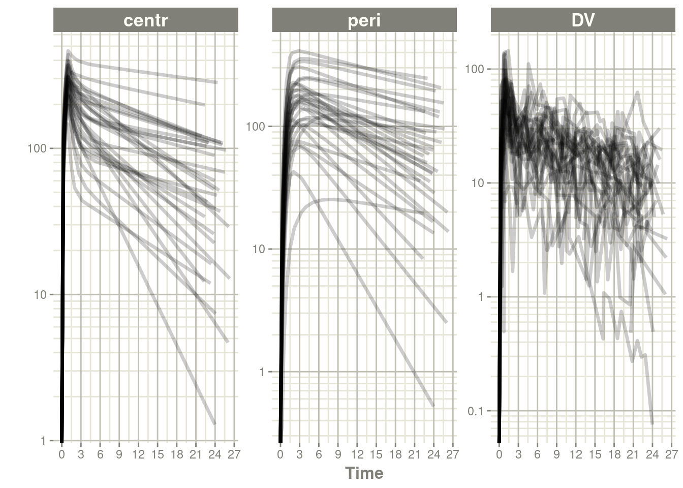

12.4.5 Daptomycin Reference

This weight-based simulation is adapted from the Daptomycin article below:

Dvorchik B, Arbeit RD, Chung J, Liu S, Knebel W, Kastrissios H. Population pharmacokinetics of daptomycin. Antimicrob Agents Che mother 2004; 48: 2799-2807. doi:(10.1128/AAC.48.8.2799-2807.2004)[https://dx.doi.org/10.1128%2FAAC.48.8.2799-2807.2004]

This simulation example was made available from the work of Sherwin Sy with modifications by Matthew Fidler

12.5 Inter-occasion and other nesting examples

More than one level of nesting is possible in rxode2; In this example we will be using the following uncertainties and sources of variability:

Level	Variable	Matrix specified	Integrated Matrix
Model uncertainty	NA	thetaMat	thetaMat
Investigator	inv.Cl, inv.Ka	omega	theta
Subject	eta.Cl, eta.Ka	omega	omega
Eye	eye.Cl, eye.Ka	omega	omega
Occasion	iov.Cl, occ.Ka	omega	omega
Unexplained Concentration	prop.sd	sigma	sigma
Unexplained Effect	add.sd	sigma	sigma

12.5.1 Event table

This event table contains nesting variables:

• inv: investigator id
• id: subject id
• eye: eye id (left or right)
• occ: occasion

library(rxode2)
library(dplyr)

et(amountUnits="mg", timeUnits="hours") %>%
  et(amt=10000, addl=9,ii=12,cmt="depot") %>%
  et(time=120, amt=2000, addl=4, ii=14, cmt="depot") %>%
  et(seq(0, 240, by=4)) %>% # Assumes sampling when there is no dosing information
  et(seq(0, 240, by=4) + 0.1) %>% ## adds 0.1 for separate eye
  et(id=1:20) %>%
  ## Add an occasion per dose
  mutate(occ=cumsum(!is.na(amt))) %>%
  mutate(occ=ifelse(occ == 0, 1, occ)) %>%
  mutate(occ=2- occ %% 2) %>%
  mutate(eye=ifelse(round(time) == time, 1, 2)) %>%
  mutate(inv=ifelse(id < 10, 1, 2)) %>% as_tibble ->
  ev

12.5.2 rxode2 model

This creates the rxode2 model with multi-level nesting. Note the variables inv.Cl, inv.Ka, eta.Cl etc; You only need one variable for each level of nesting.

mod <- rxode2({
  ## Clearance with individuals
  eff(0) = 1
  C2 = centr/V2*(1+prop.sd)
  C3 = peri/V3
  CL =  TCl*exp(eta.Cl + eye.Cl + iov.Cl + inv.Cl)
  KA = TKA * exp(eta.Ka + eye.Ka + iov.Cl + inv.Ka)
  d/dt(depot) =-KA*depot
  d/dt(centr) = KA*depot - CL*C2 - Q*C2 + Q*C3
  d/dt(peri)  =                    Q*C2 - Q*C3
  d/dt(eff)  = Kin - Kout*(1-C2/(EC50+C2))*eff
  ef0 = eff + add.sd
})

#> using C compiler: ‘gcc (Ubuntu 11.4.0-1ubuntu1~22.04) 11.4.0’

12.5.3 Uncertainty in Model parameters

theta <- c("TKA"=0.294, "TCl"=18.6, "V2"=40.2,
           "Q"=10.5, "V3"=297, "Kin"=1, "Kout"=1, "EC50"=200)

## Creating covariance matrix
tmp <- matrix(rnorm(8^2), 8, 8)
tMat <- tcrossprod(tmp, tmp) / (8 ^ 2)
dimnames(tMat) <- list(names(theta), names(theta))

tMat

#>                TKA         TCl            V2             Q           V3
#> TKA   1.408151e-01  0.08277499  0.0180178917 -0.0470325576  0.029172564
#> TCl   8.277499e-02  0.18104452 -0.0532724661 -0.0421074920  0.068093695
#> V2    1.801789e-02 -0.05327247  0.0581816756  0.0001167516  0.006496495
#> Q    -4.703256e-02 -0.04210749  0.0001167516  0.1549374667  0.020764042
#> V3    2.917256e-02  0.06809370  0.0064964951  0.0207640421  0.118986685
#> Kin  -3.445136e-02  0.01464937 -0.0426405263  0.1503174753 -0.039702872
#> Kout -2.904363e-02 -0.04914350  0.0324790929  0.0069332072  0.030349396
#> EC50 -4.017336e-05  0.02850637 -0.0326094799 -0.0489119232 -0.029606732
#>               Kin         Kout          EC50
#> TKA  -0.034451357 -0.029043632 -4.017336e-05
#> TCl   0.014649373 -0.049143503  2.850637e-02
#> V2   -0.042640526  0.032479093 -3.260948e-02
#> Q     0.150317475  0.006933207 -4.891192e-02
#> V3   -0.039702872  0.030349396 -2.960673e-02
#> Kin   0.299597107 -0.074421154 -6.528526e-03
#> Kout -0.074421154  0.061039604 -2.800741e-02
#> EC50 -0.006528526 -0.028007407  4.167429e-02

12.5.4 Nesting Variability

To specify multiple levels of nesting, you can specify it as a nested lotri matrix; When using this approach you use the condition operator | to specify what variable nesting occurs on; For the Bayesian simulation we need to specify how much information we have for each parameter; For rxode2 this is the nu parameter.

In this case: - id, nu=100 or the model came from 100 subjects - eye, nu=200 or the model came from 200 eyes - occ, nu=200 or the model came from 200 occasions - inv, nu=10 or the model came from 10 investigators

To specify this in lotri you can use | var(nu=X), or:

omega <- lotri(lotri(eta.Cl ~ 0.1,
                     eta.Ka ~ 0.1) | id(nu=100),
               lotri(eye.Cl ~ 0.05,
                     eye.Ka ~ 0.05) | eye(nu=200),
               lotri(iov.Cl ~ 0.01,
                     iov.Ka ~ 0.01) | occ(nu=200),
               lotri(inv.Cl ~ 0.02,
                     inv.Ka ~ 0.02) | inv(nu=10))
omega

#> $id
#>        eta.Cl eta.Ka
#> eta.Cl    0.1    0.0
#> eta.Ka    0.0    0.1
#> 
#> $eye
#>        eye.Cl eye.Ka
#> eye.Cl   0.05   0.00
#> eye.Ka   0.00   0.05
#> 
#> $occ
#>        iov.Cl iov.Ka
#> iov.Cl   0.01   0.00
#> iov.Ka   0.00   0.01
#> 
#> $inv
#>        inv.Cl inv.Ka
#> inv.Cl   0.02   0.00
#> inv.Ka   0.00   0.02
#> 
#> Properties: nu

12.5.5 Unexplained variability

The last piece of variability to specify is the unexplained variability

sigma <- lotri(prop.sd ~ .25,
               add.sd~ 0.125)

12.5.6 Solving the problem

s <- rxSolve(mod, theta, ev,
             thetaMat=tMat, omega=omega,
             sigma=sigma, sigmaDf=400,
             nStud=400)

#> using C compiler: ‘gcc (Ubuntu 11.4.0-1ubuntu1~22.04) 11.4.0’

#> unhandled error message: EE:[lsoda] 70000 steps taken before reaching tout
#>  @(lsoda.c:750

#> Warning: some ID(s) could not solve the ODEs correctly; These values are
#> replaced with 'NA'

print(s)

#> -- Solved rxode2 object --
#> -- Parameters ($params): --
#> # A tibble: 8,000 x 24
#>    sim.id id    `inv.Cl(inv==1)` `inv.Cl(inv==2)` `inv.Ka(inv==1)`
#>     <int> <fct>            <dbl>            <dbl>            <dbl>
#>  1      1 1                0.251           0.0765          -0.0741
#>  2      1 2                0.251           0.0765          -0.0741
#>  3      1 3                0.251           0.0765          -0.0741
#>  4      1 4                0.251           0.0765          -0.0741
#>  5      1 5                0.251           0.0765          -0.0741
#>  6      1 6                0.251           0.0765          -0.0741
#>  7      1 7                0.251           0.0765          -0.0741
#>  8      1 8                0.251           0.0765          -0.0741
#>  9      1 9                0.251           0.0765          -0.0741
#> 10      1 10               0.251           0.0765          -0.0741
#> # i 7,990 more rows
#> # i 19 more variables: `inv.Ka(inv==2)` <dbl>, `eye.Cl(eye==1)` <dbl>,
#> #   `eye.Cl(eye==2)` <dbl>, `eye.Ka(eye==1)` <dbl>, `eye.Ka(eye==2)` <dbl>,
#> #   `iov.Cl(occ==1)` <dbl>, `iov.Cl(occ==2)` <dbl>, `iov.Ka(occ==1)` <dbl>,
#> #   `iov.Ka(occ==2)` <dbl>, V2 <dbl>, V3 <dbl>, TCl <dbl>, eta.Cl <dbl>,
#> #   TKA <dbl>, eta.Ka <dbl>, Q <dbl>, Kin <dbl>, Kout <dbl>, EC50 <dbl>
#> -- Initial Conditions ($inits): --
#> depot centr  peri   eff 
#>     0     0     0     1 
#> 
#> Simulation with uncertainty in:
#> * parameters ($thetaMat for changes)
#> * omega matrix ($omegaList)
#> 
#> -- First part of data (object): --
#> # A tibble: 976,000 x 21
#>   sim.id    id time inv.Cl  inv.Ka eye.Cl  eye.Ka   iov.Cl iov.Ka     C2     C3
#>    <int> <int>  [h]  <dbl>   <dbl>  <dbl>   <dbl>    <dbl>  <dbl>  <dbl>  <dbl>
#> 1      1     1  0    0.251 -0.0741 0.0127 -0.156  -0.00963 0.0813  0     0     
#> 2      1     1  0.1  0.251 -0.0741 0.122  -0.0143 -0.00963 0.0813 13.5   0.0159
#> 3      1     1  4    0.251 -0.0741 0.0127 -0.156  -0.00963 0.0813  2.36  3.80  
#> 4      1     1  4.1  0.251 -0.0741 0.122  -0.0143 -0.00963 0.0813  8.16  3.84  
#> 5      1     1  8    0.251 -0.0741 0.0127 -0.156  -0.00963 0.0813  0.392 4.26  
#> 6      1     1  8.1  0.251 -0.0741 0.122  -0.0143 -0.00963 0.0813  0.728 4.25  
#> # i 975,994 more rows
#> # i 10 more variables: CL <dbl>, KA <dbl>, ef0 <dbl>, depot <dbl>, centr <dbl>,
#> #   peri <dbl>, eff <dbl>, occ <fct>, eye <fct>, inv <fct>

There are multiple investigators in a study; Each investigator has a number of individuals enrolled at their site. rxode2 automatically determines the number of investigators and then will simulate an effect for each investigator. With the output, inv.Cl(inv==1) will be the inv.Cl for investigator 1, inv.Cl(inv==2) will be the inv.Cl for investigator 2, etc.

inv.Cl(inv==1), inv.Cl(inv==2), etc will be simulated for each study and then combined to form the between investigator variability. In equation form these represent the following:

inv.Cl = (inv == 1) * `inv.Cl(inv==1)` + (inv == 2) * `inv.Cl(inv==2)`

If you look at the simulated parameters you can see inv.Cl(inv==1) and inv.Cl(inv==2) are in the s$params; They are the same for each study:

print(head(s$params))

#>   sim.id id inv.Cl(inv==1) inv.Cl(inv==2) inv.Ka(inv==1) inv.Ka(inv==2)
#> 1      1  1      0.2511322     0.07650072    -0.07407926     0.02202168
#> 2      1  2      0.2511322     0.07650072    -0.07407926     0.02202168
#> 3      1  3      0.2511322     0.07650072    -0.07407926     0.02202168
#> 4      1  4      0.2511322     0.07650072    -0.07407926     0.02202168
#> 5      1  5      0.2511322     0.07650072    -0.07407926     0.02202168
#> 6      1  6      0.2511322     0.07650072    -0.07407926     0.02202168
#>   eye.Cl(eye==1) eye.Cl(eye==2) eye.Ka(eye==1) eye.Ka(eye==2) iov.Cl(occ==1)
#> 1     0.01270627     0.12170298    -0.15645931    -0.01431089   -0.009629471
#> 2    -0.17730664     0.03257883     0.32307021     0.02920050   -0.174327268
#> 3     0.11662407     0.23070953     0.14031942     0.60774555    0.108968491
#> 4     0.15094002    -0.06667588     0.14962819     0.06226514   -0.043479003
#> 5    -0.03450830     0.18531423    -0.52570577    -0.14201201   -0.062005657
#> 6    -0.35488059     0.58910822    -0.05440263     0.01390173   -0.032395527
#>   iov.Cl(occ==2) iov.Ka(occ==1) iov.Ka(occ==2)       V2       V3      TCl
#> 1     0.01053195    0.081266104    -0.07738340 39.89608 296.4477 18.66578
#> 2     0.14111236    0.012959501     0.14003903 39.89608 296.4477 18.66578
#> 3    -0.08081801    0.064904438    -0.05309035 39.89608 296.4477 18.66578
#> 4    -0.02781613    0.021622026    -0.17969560 39.89608 296.4477 18.66578
#> 5     0.14666663   -0.032748073    -0.02417555 39.89608 296.4477 18.66578
#> 6    -0.02895152    0.002390472     0.05844429 39.89608 296.4477 18.66578
#>       eta.Cl      TKA      eta.Ka        Q        Kin      Kout    EC50
#> 1  0.6985427 0.346799  0.42017137 9.659552 0.03348837 0.9102127 200.427
#> 2 -0.1405521 0.346799 -0.17769437 9.659552 0.03348837 0.9102127 200.427
#> 3  0.2575912 0.346799  0.22284272 9.659552 0.03348837 0.9102127 200.427
#> 4  0.4722423 0.346799  0.49685712 9.659552 0.03348837 0.9102127 200.427
#> 5 -0.1505078 0.346799 -0.43312621 9.659552 0.03348837 0.9102127 200.427
#> 6 -0.1271020 0.346799  0.08195574 9.659552 0.03348837 0.9102127 200.427

print(head(s$params %>% filter(sim.id == 2)))

#>   sim.id id inv.Cl(inv==1) inv.Cl(inv==2) inv.Ka(inv==1) inv.Ka(inv==2)
#> 1      2  1      0.1093052     -0.0673165      0.1186236    -0.08942504
#> 2      2  2      0.1093052     -0.0673165      0.1186236    -0.08942504
#> 3      2  3      0.1093052     -0.0673165      0.1186236    -0.08942504
#> 4      2  4      0.1093052     -0.0673165      0.1186236    -0.08942504
#> 5      2  5      0.1093052     -0.0673165      0.1186236    -0.08942504
#> 6      2  6      0.1093052     -0.0673165      0.1186236    -0.08942504
#>   eye.Cl(eye==1) eye.Cl(eye==2) eye.Ka(eye==1) eye.Ka(eye==2) iov.Cl(occ==1)
#> 1     0.35152729    0.006594725    -0.06268297     0.29815635    -0.00881754
#> 2     0.10269092    0.146594486    -0.20490974     0.28538009    -0.07747854
#> 3    -0.63206970    0.346871624     0.06642099     0.35270304    -0.06741916
#> 4    -0.08415895    0.235107634     0.12953250    -0.17707732     0.06017794
#> 5     0.33726812    0.072669926    -0.05740940    -0.08718347    -0.09088558
#> 6    -0.26619889   -0.007725891    -0.18858394    -0.15278522     0.14865110
#>   iov.Cl(occ==2) iov.Ka(occ==1) iov.Ka(occ==2)       V2       V3      TCl
#> 1    0.015905350    -0.02096693    -0.12871823 39.95281 297.0105 18.48517
#> 2    0.021713327     0.10111395    -0.04911822 39.95281 297.0105 18.48517
#> 3   -0.027550757    -0.08063562     0.07982127 39.95281 297.0105 18.48517
#> 4   -0.019521504     0.06468350     0.08335715 39.95281 297.0105 18.48517
#> 5   -0.003415422    -0.03601159     0.04816064 39.95281 297.0105 18.48517
#> 6   -0.053526809    -0.16281362     0.01215932 39.95281 297.0105 18.48517
#>        eta.Cl        TKA      eta.Ka        Q      Kin      Kout     EC50
#> 1 -0.35476449 -0.1722565  0.21079536 10.89209 1.256925 0.9366159 199.9913
#> 2 -0.17388248 -0.1722565  0.62943162 10.89209 1.256925 0.9366159 199.9913
#> 3  0.90160059 -0.1722565  0.08201732 10.89209 1.256925 0.9366159 199.9913
#> 4  0.10391092 -0.1722565  0.38871734 10.89209 1.256925 0.9366159 199.9913
#> 5  0.28247914 -0.1722565 -0.14271404 10.89209 1.256925 0.9366159 199.9913
#> 6 -0.02269591 -0.1722565  0.29263333 10.89209 1.256925 0.9366159 199.9913

For between eye variability and between occasion variability each individual simulates a number of variables that become the between eye and between occasion variability; In the case of the eye:

eye.Cl = (eye == 1) * `eye.Cl(eye==1)` + (eye == 2) * `eye.Cl(eye==2)`

So when you look the simulation each of these variables (ie eye.Cl(eye==1), eye.Cl(eye==2), etc) they change for each individual and when combined make the between eye variability or the between occasion variability that can be seen in some pharamcometric models.

12.6 Transit compartment models

Savic 2008 first introduced the idea of transit compartments being a mechanistic explanation of a a lag-time type phenomena. rxode2 has special handling of these models:

You can specify this in a similar manner as the original paper:

library(rxode2)

mod <- function() {
  model({
    ## Table 3 from Savic 2007
    cl = 17.2 # (L/hr)
    vc = 45.1 # L
    ka = 0.38 # 1/hr
    mtt = 0.37 # hr
    bio=1
    n = 20.1
    k = cl/vc
    ktr = (n+1)/mtt
    ## note that lgammafn is the same as lgamma in R.
    d/dt(depot) = exp(log(bio*podo(depot))+log(ktr)+n*log(ktr*tad(depot))-
                        ktr*tad(depot)-lgammafn(n+1))-ka*depot
    d/dt(cen) = ka*depot-k*cen
  })
}

et <- et(0, 7, length.out=200) %>%
  et(amt=20, time=0, evid=7)

transit <- rxSolve(mod, et)

#> using C compiler: ‘gcc (Ubuntu 11.4.0-1ubuntu1~22.04) 11.4.0’

plot(transit, cen, ylab="Central Concentration")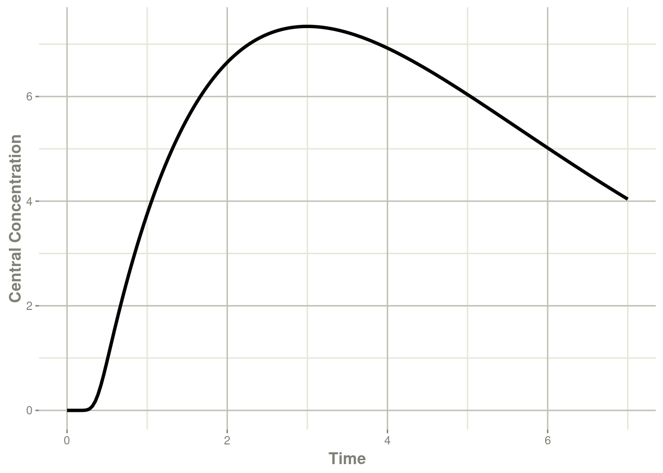

Another option is to specify the transit compartment function transit syntax. This specifies the parameters transit(number of transit compartments, mean transit time, bioavailability). The bioavailability term is optional.

The same model can be specified by:

mod <- function() {
  ini({
    ## Table 3 from Savic 2007
    cl  <- 17.2 # (L/hr)
    vc  <- 45.1 # L
    ka  <- 0.38 # 1/hr
    mtt <- 0.37 # hr
    bio <- 1
    n   <- 20.1
  })
  model({
    k           <- cl/vc
    ktr         <- (n+1)/mtt
    d/dt(depot) <- transit(n,mtt,bio)-ka*depot
    d/dt(cen)   <- ka*depot-k*cen
  })
}

et <- et(0, 7, length.out=200) %>%
  et(amt=20, evid=7)

transit <- rxSolve(mod, et)

#> i parameter labels from comments will be replaced by 'label()'

#> using C compiler: ‘gcc (Ubuntu 11.4.0-1ubuntu1~22.04) 11.4.0’

plot(transit, cen, ylab="Central Concentration")

A couple of things to keep in mind when using this approach:

• This approach implicitly assumes that the absorption through the transit compartment is completed before the next dose begins

• Different types of doses (ie bolus/infusion) to the compartment affect the time after dose calculation (tad) which is used in the transit compartment calculation. These (therefore) are not currently supported. The most stable way is to use tad(cmt) and podo(cmt), this way doses to other compartments do not affect the transit compartment calculation.

• Internally, the transit syntax uses either the currently defined cmt d/dt(cmt)=transit(...), or cmt. If the transit compartment is used outside of a d/dt() (not recommended), the cmt that is used is the last d/dt(cmt) defined it the model. This also means compartments do not affect one another (ie a oral, transit compartment drug dosed immediately with an IV infusion)