Converting Monolix fit to nlmixr2 fit
Source:vignettes/articles/convert-nlmixr2.Rmd
convert-nlmixr2.RmdCreating a nlmixr2 compatible model
Unlike nonmem2rx, the residuals specification can be
converted more efficiently to the nlmixr2 residual syntax.
Example
library(babelmixr2) # will re-export much of monolix2rx

# You use the path to the monolix mlxtran file

# In this case we will us the theophylline project included in monolix2rx
pkgTheo <- system.file("theo/theophylline_project.mlxtran", package="monolix2rx")

# Note you have to setup monolix2rx to use the model library or save the model as a separate file
mod <- monolix2rx(pkgTheo)
#> ℹ integrated model file 'oral1_1cpt_kaVCl.txt' into mlxtran object
#> ℹ updating model values to final parameter estimates
#> ℹ done
#> ℹ reading run info (# obs, doses, Monolix Version, etc) from summary.txt
#> ℹ done
#> ℹ reading covariance from FisherInformation/covarianceEstimatesLin.txt
#> ℹ done
#> Warning in .dataRenameFromMlxtran(data, .mlxtran): NAs introduced by coercion
#> ℹ imported monolix and translated to rxode2 compatible data ($monolixData)
#> ℹ imported monolix ETAS (_SAEM) imported to rxode2 compatible data ($etaData)
#> ℹ imported monolix pred/ipred data to compare ($predIpredData)
#> ℹ solving ipred problem
#> ℹ done
#> ℹ solving pred problem
#> ℹ done

print(mod)
#>  ── rxode2-based free-form 2-cmt ODE model ──────────────────────────────────────
#>  ── Initalization: ──
#> Fixed Effects ($theta):
#>      ka_pop       V_pop      Cl_pop           a           b
#>  0.42699448 -0.78635157 -3.21457598  0.43327956  0.05425953
#>
#> Omega ($omega):
#>           omega_ka    omega_V   omega_Cl
#> omega_ka 0.4503145 0.00000000 0.00000000
#> omega_V  0.0000000 0.01594701 0.00000000
#> omega_Cl 0.0000000 0.00000000 0.07323701
#>
#> States ($state or $stateDf):
#>   Compartment Number Compartment Name
#> 1                  1            depot
#> 2                  2          central
#>  ── μ-referencing ($muRefTable): ──
#>    theta      eta level
#> 1 ka_pop omega_ka    id
#> 2  V_pop  omega_V    id
#> 3 Cl_pop omega_Cl    id
#>
#>  ── Model (Normalized Syntax): ──
#> function() {
#>     description <- "The administration is extravascular with a first order absorption (rate constant ka).\nThe PK model has one compartment (volume V) and a linear elimination (clearance Cl).\nThis has been modified so that it will run without the model library"
#>     dfObs <- 120
#>     dfSub <- 12
#>     thetaMat <- lotri({
#>         ka_pop ~ 0.09785
#>         V_pop ~ c(0.00082606, 0.00041937)
#>         Cl_pop ~ c(-4.2833e-05, -6.7957e-06, 1.1318e-05)
#>         omega_ka ~ c(omega_ka = 0.022259)
#>         omega_V ~ c(omega_ka = -7.6443e-05, omega_V = 0.0014578)
#>         omega_Cl ~ c(omega_ka = 3.062e-06, omega_V = -1.2912e-05,
#>             omega_Cl = 0.0039578)
#>         a ~ c(omega_ka = -0.0001227, omega_V = -6.5914e-05, omega_Cl = -0.00041194,
#>             a = 0.015333)
#>         b ~ c(omega_ka = -1.3886e-05, omega_V = -3.1105e-05,
#>             omega_Cl = 5.2805e-05, a = -0.0026458, b = 0.00056232)
#>     })
#>     validation <- c("ipred relative difference compared to Monolix ipred: 0.04%; 95% percentile: (0%,0.52%); rtol=0.00038",
#>         "ipred absolute difference compared to Monolix ipred: 95% percentile: (0.000362, 0.00848); atol=0.00254",
#>         "pred relative difference compared to Monolix pred: 0%; 95% percentile: (0%,0%); rtol=6.6e-07",
#>         "pred absolute difference compared to Monolix pred: 95% percentile: (1.6e-07, 1.27e-05); atol=3.66e-06",
#>         "iwres relative difference compared to Monolix iwres: 0%; 95% percentile: (0.06%,32.22%); rtol=0.0153",
#>         "iwres absolute difference compared to Monolix pred: 95% percentile: (0.000403, 0.0138); atol=0.00305")
#>     ini({
#>         ka_pop <- 0.426994483535611
#>         V_pop <- -0.786351566327091
#>         Cl_pop <- -3.21457597916301
#>         a <- c(0, 0.433279557549051)
#>         b <- c(0, 0.0542595276206251)
#>         omega_ka ~ 0.450314511978718
#>         omega_V ~ 0.0159470121255372
#>         omega_Cl ~ 0.0732370098834837
#>     })
#>     model({
#>         cmt(depot)
#>         cmt(central)
#>         ka <- exp(ka_pop + omega_ka)
#>         V <- exp(V_pop + omega_V)
#>         Cl <- exp(Cl_pop + omega_Cl)
#>         d/dt(depot) <- -ka * depot
#>         d/dt(central) <- +ka * depot - Cl/V * central
#>         Cc <- central/V
#>         CONC <- Cc
#>         CONC ~ add(a) + prop(b) + combined1()
#>     })
#> }
Converting the model to a nlmixr2 fit
Once you have a rxode2() model that:
Qualifies against the NONMEM model,
Has
nlmixr2compatible residuals
You can then convert it to a nlmixr2 fit object with
babelmixr2:
library(babelmixr2)
fit <- as.nlmixr2(mod)
#> → loading into symengine environment...
#> → pruning branches (`if`/`else`) of full model...
#> ✔ done
#> → finding duplicate expressions in EBE model...
#> [====|====|====|====|====|====|====|====|====|====] 0:00:00
#> → optimizing duplicate expressions in EBE model...
#> [====|====|====|====|====|====|====|====|====|====] 0:00:00
#> → compiling EBE model...
#> ✔ done
#> rxode2 5.0.2 using 2 threads (see ?getRxThreads)
#> no cache: create with `rxCreateCache()`
#> → Calculating residuals/tables
#> ✔ done
#> ℹ monolix parameter history integrated into fit object
# If you want you can use nlmixr2, to add cwres to this fit:
fit <- addCwres(fit)
#> → loading into symengine environment...
#> → pruning branches (`if`/`else`) of full model...
#> ✔ done
#> → calculate jacobian
#> [====|====|====|====|====|====|====|====|====|====] 0:00:00
#> → calculate sensitivities
#> [====|====|====|====|====|====|====|====|====|====] 0:00:00
#> → calculate ∂(f)/∂(η)
#> [====|====|====|====|====|====|====|====|====|====] 0:00:00
#> → calculate ∂(R²)/∂(η)
#> [====|====|====|====|====|====|====|====|====|====] 0:00:00
#> → finding duplicate expressions in inner model...
#> [====|====|====|====|====|====|====|====|====|====] 0:00:00
#> → optimizing duplicate expressions in inner model...
#> [====|====|====|====|====|====|====|====|====|====] 0:00:00
#>
#> [====|====|====|====|====|====|====|====|====|====] 0:00:00
#>
#> [====|====|====|====|====|====|====|====|====|====] 0:00:00
#> → finding duplicate expressions in EBE model...
#> [====|====|====|====|====|====|====|====|====|====] 0:00:00
#> → optimizing duplicate expressions in EBE model...
#> [====|====|====|====|====|====|====|====|====|====] 0:00:00
#> → compiling inner model...
#> ✔ done
#> → finding duplicate expressions in FD model...
#> [====|====|====|====|====|====|====|====|====|====] 0:00:00
#> → optimizing duplicate expressions in FD model...
#> [====|====|====|====|====|====|====|====|====|====] 0:00:00
#> → compiling EBE model...
#> ✔ done
#> → compiling events FD model...
#> ✔ done
#> → Calculating residuals/tables
#> ✔ done
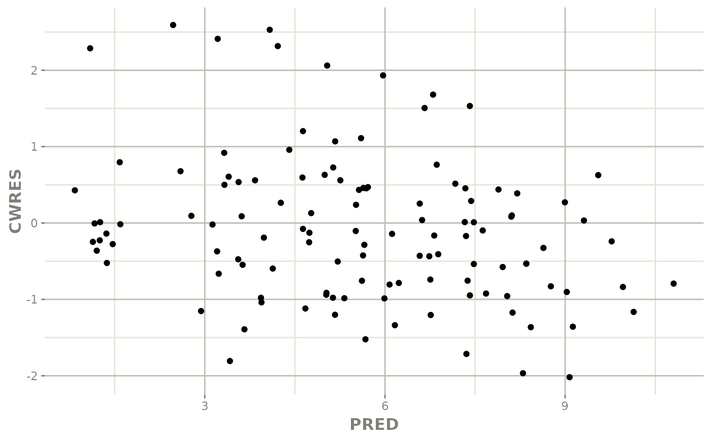
library(ggplot2)
ggplot(fit, aes(PRED, CWRES)) +
geom_point() + rxode2::rxTheme()