nlmixr2 Algebraic Solutions with Formula

Bill Denney

2026-09-11

Introduction

Some models are able to be described by simple algebraic solutions. To simplify algebraic models, you can use a formula interface similar to the formula used with the lme4 library. (The formula interface is described in more detail below; knowledge of lme4 is not required to use the formula interface.)

Quick start

The simplest, non-trivial model is a linear model, y = m*x + b. We will generate the data for this model and then fit it to show the simplest use case of the nlmixr2 formula interface.

library(nlmixr2extra)
library(dplyr)
#> 
#> Attaching package: 'dplyr'
#> The following objects are masked from 'package:stats':
#> 
#>     filter, lag
#> The following objects are masked from 'package:base':
#> 
#>     intersect, setdiff, setequal, union
library(ggplot2)

# Simulate the equation y = 3*x + 5 with normally-distributed residual error
# having a standard deviation of 5
withr::with_seed(
  5, # standardize the random seed so that the results are reproducible
  dSim <-
    data.frame(
      x = 1:100,
      y =
        (1:100)*3 +
        5 +
        rnorm(n = 100, mean = 0, sd = 5)
    )
)

ggplot(dSim, aes(x=x, y=y)) + geom_point()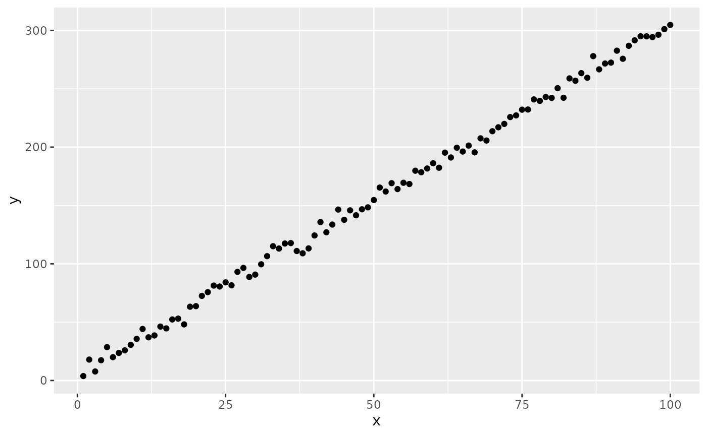

To fit this model requires only one line of R code:

modLm :=
  nlmixrFormula(
    y~m*x + b,
    data = dSim,
    start = c(m = 2.5, b = 4, addSd = 2),
    est = "focei"
  )
#> ℹ loading fit from nlmixrFormula-modLm.zip
#> ℹ loading fit from modLm.R
#> ℹ parameter labels from comments are typically ignored in non-interactive mode
#> ℹ Need to run with the source intact to parse comments
#> ℹ removing unzipped fit files

You can also use a call to nlmixr or nlmixr2, the arguments are the same as nlmixrFormula:

modLm2 :=
  nlmixr(
    y ~ m*x + b,
    data = dSim,
    start = c(m = 2.5, b = 4, addSd = 2),
    est = "focei"
  )
#> ℹ loading fit from nlmixrFormula-modLm2.zip
#> ℹ loading fit from modLm2.R
#> ℹ parameter labels from comments are typically ignored in non-interactive mode
#> ℹ Need to run with the source intact to parse comments
#> ℹ removing unzipped fit files

Quick start, mixed-effects model

A more typical use case for nlmixr2 is a mixed-effects model. It adds (subject-level) random effects to the model.

# Setup the dataset for nonlinear mixed-effects fitting

# Simulate the equation y = 3*x + 5 with normally-distributed residual error
# having a standard deviation of 5
withr::with_seed(
  5, # standardize the random seed so that the results are reproducible
  {
    dSimSetup <-
      data.frame(
        id = rep(1:10, each=10),
        x = rep(1:10, 10),
        y = 1
      )
    dSimNlmePrep <-
      nlmixrFormula(
        y~m*x + b + bRe ~ bRe|id,
        start = c(m=3, b=5, addSd=5),
        data = dSimSetup,
        est = "rxSolve"
      )
  }
)
#> ℹ parameter labels from comments are typically ignored in non-interactive mode
#> ℹ Need to run with the source intact to parse comments

# Modify the simulated results to be ready for fitting
dSimNlme <-
  dSimNlmePrep |>
  as.data.frame() |>
  select(id, time, x, y=sim)

ggplot(dSimNlme, aes(x=x, y=y, colour=factor(id))) + geom_point()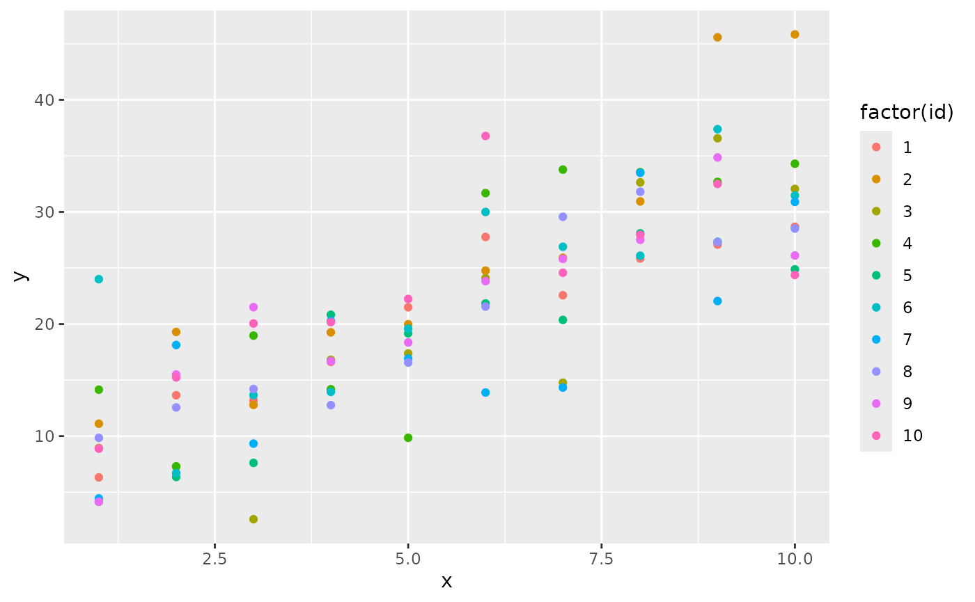

modNlme :=
  nlmixr(
    y~m*x + b + bRe ~ bRe|id,
    start = c(m=3, b=5, addSd=5),
    data = dSimNlme,
    est = "focei"
  )
#> ℹ loading fit from nlmixrFormula-modNlme.zip
#> ℹ loading fit from modNlme.R
#> ℹ parameter labels from comments are typically ignored in non-interactive mode
#> ℹ Need to run with the source intact to parse comments
#> ℹ removing unzipped fit files

modNlme

$$\begin{align*} {value} & = {m} {\times} {x}+{b}+{bRe} \\ {value} & \sim add({addSd}) \end{align*}$$

In this model, the fixed effects of m and b were estimated along with the random effect of bRe.

Quick start, automatic parameter fixed effects

# Setup the dataset for nonlinear mixed-effects fitting with different types of
# parameters.

# Simulate the equation y = 3*x + 4(when z = 'a') or 6(when z = 'b') with normally-distributed residual error
# having a standard deviation of 5
withr::with_seed(
  5, # standardize the random seed so that the results are reproducible
  {
    dSimSetup <-
      data.frame(
        id = rep(1:10, each=10),
        x = rep(1:10, 10),
        y = 1,
        z = sample(factor(c("a", "b")), size = 100, replace = TRUE)
      )
    # Note that we need to give `start` as a list so that `b` can carry one
    # starting value per factor level of `z` (named-vector `c()` cannot hold
    # multi-element entries).
    dSimNlmePrep <-
      nlmixrFormula(
        y~m*x + b + bRe ~ bRe|id,
        start = list(m=3, b=c(4, 2), addSd=5),
        param = list(b ~ z),
        data = dSimSetup,
        est = "rxSolve"
      )
  }
)
#> ℹ parameter labels from comments are typically ignored in non-interactive mode
#> ℹ Need to run with the source intact to parse comments

# Modify the simulated results to be ready for fitting
dSimNlme <-
  dSimNlmePrep |>
  as.data.frame() |>
  select(id, time, x, y=sim, z)

ggplot(dSimNlme, aes(x=x, y=y, colour=z)) +
  geom_point() +
  geom_line(aes(group = id), colour = "gray")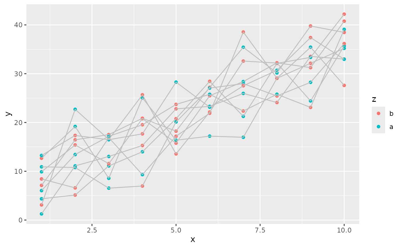

modParam :=
  nlmixr(
    y~m*x + b + bRe ~ bRe|id,
    start = list(m=3, b=c(4, 2), addSd=5),
    param = list(b ~ z),
    data = dSimNlme,
    est = "focei"
  )
#> ℹ loading fit from nlmixrFormula-modParam.zip
#> ℹ loading fit from modParam.R
#> ℹ parameter labels from comments are typically ignored in non-interactive mode
#> ℹ Need to run with the source intact to parse comments
#> ℹ removing unzipped fit files

modParam

$$\begin{align*} {b} & = {b.z.b}+{b.z.a} {\times} \left({z}{\equiv}\text{"a"}\right) \\ {value} & = {m} {\times} {x}+{b}+{bRe} \\ {value} & \sim add({addSd}) \end{align*}$$

Quick start, continuous covariate on a parameter

param also accepts numeric (continuous) covariate columns. When b is modelled as a linear function of a continuous covariate w, two parameters are introduced: pop.b (the intercept) and cov_w_b (the slope on w). The generated model line is b <- pop.b + cov_w_b * w.

start[["b"]] may be a single value (treated as the intercept; the slope starts at 0) or c(intercept, slope).

withr::with_seed(
  5,
  {
    dSimSetup <-
      data.frame(
        id = rep(1:10, each=10),
        x = rep(1:10, 10),
        y = 1,
        w = runif(100, min = 0, max = 10)
      )
    dSimContPrep <-
      nlmixrFormula(
        y~m*x + b + bRe ~ bRe|id,
        start = list(m=3, b=c(4, 0.2), addSd=5),
        param = list(b ~ w),
        data = dSimSetup,
        est = "rxSolve"
      )
  }
)
#> ℹ parameter labels from comments are typically ignored in non-interactive mode
#> ℹ Need to run with the source intact to parse comments

dSimCont <-
  dSimContPrep |>
  as.data.frame() |>
  select(id, time, x, w, y=sim)

modCont :=
  nlmixr(
    y~m*x + b + bRe ~ bRe|id,
    start = list(m=3, b=c(4, 0.2), addSd=5),
    param = list(b ~ w),
    data = dSimCont,
    est = "focei"
  )
#> ℹ loading fit from nlmixrFormula-modCont.zip
#> ℹ loading fit from modCont.R
#> ℹ parameter labels from comments are typically ignored in non-interactive mode
#> ℹ Need to run with the source intact to parse comments
#> ℹ removing unzipped fit files

modCont

$$\begin{align*} {b} & = {pop.b}+{cov\_w\_b} {\times} {w} \\ {value} & = {m} {\times} {x}+{b}+{bRe} \\ {value} & \sim add({addSd}) \end{align*}$$

Quick start, log-linked parameter

Some parameters are naturally strictly positive (clearances, volumes, rate constants). Pass paramLink = c(<parameter> = "log") to wrap the linear combination in exp(). The starting values are then on the log scale.

nlmixr(
  y~m*x + b + bRe ~ bRe|id,
  start = list(m=3, b=c(log(4), 0.2), addSd=5),
  param = list(b ~ w),
  paramLink = c(b = "log"),
  data = dSimCont,
  est = "focei"
)

Worked example: concentration-QT analysis

A common use of the formula interface is a thorough QT (TQT) or concentration-QT (C-QT) analysis. The clinical question is whether a 10 msec $\Delta QT$ is exceeded at therapeutic drug concentrations. The standard model has:

• A categorical effect for nominal post-dose time (captures circadian and food-related drift)
• A continuous linear effect for drug concentration (the parameter of interest)
• A per-subject random intercept (baseline $\Delta QT$ offset)

In the formula interface this is one call:

dQT ~ b + bRe ~ (bRe|id)
param  = list(b ~ timeF + conc)

b is a single intercept parameter; param decomposes it into a fixed effect per timeF level plus a linear slope on conc. The random per- subject offset bRe is added to b in the predictor.

Simulating the data

We start from a one-compartment oral PK profile (Bateman equation), scale it so the typical $C_{max}$ is about 1000 ng/mL, and apply per-subject log-normal scaling so individual $C_{max}$ values are log-normally distributed.

withr::with_seed(42, {
  nSubj    <- 40
  nomTimes <- c(0, 0.5, 1, 1.5, 2, 3, 4, 6, 8, 12)  # 10 nominal times

  # Typical 1-compartment oral PK profile (unit Bateman), then scaled
  # so the population Cmax is 1000 ng/mL
  bateman    <- function(t, ka = 2, ke = 0.1) {
    (ka / (ka - ke)) * (exp(-ke * t) - exp(-ka * t))
  }
  cmaxFactor <- 1000 / max(bateman(seq(0, 12, 0.01)))

  # Per-subject log-normal scaling of the concentration profile
  subjScale  <- exp(rnorm(nSubj, mean = 0, sd = 0.4))

  cqtDesign <-
    expand.grid(id = 1:nSubj, timeH = nomTimes)
  cqtDesign$conc  <- bateman(cqtDesign$timeH) * cmaxFactor *
                     subjScale[cqtDesign$id]
  cqtDesign$timeF <- factor(cqtDesign$timeH,
                            levels = as.character(nomTimes))
  cqtDesign$dQT   <- 1  # placeholder; nlmixrFormula(est="rxSolve") fills it in
})

Now we simulate dQT from the true model. The true slope is 0.01 msec/(ng/mL), which produces about a 10 msec $\Delta QT$ at the population $C_{max}$. The categorical time effects encode a typical circadian drift pattern. The simulation’s bRe SD is 1 (the formula interface’s current default for random-effect starting values).

cqtSimPrep <-
  nlmixrFormula(
    dQT ~ b + bRe ~ (bRe|id),
    data  = cqtDesign,
    # 10 time-level intercepts (relative to time 0) + slope on conc
    start = list(
      b     = c(0,         # timeF == 0  (pre-dose baseline)
                3, 5, 6, 5, 2, 0, -1, -2, -3,  # post-dose time effects
                0.01),     # slope on conc (msec per ng/mL)
      addSd = 3
    ),
    param = list(b ~ timeF + conc),
    est   = "rxSolve"
  )
#> ℹ parameter labels from comments are typically ignored in non-interactive mode
#> ℹ Need to run with the source intact to parse comments

cqtData <-
  cqtSimPrep |>
  as.data.frame() |>
  select(id, conc, timeF, dQT = sim)

ggplot(cqtData, aes(x = conc, y = dQT, colour = timeF)) +
  geom_point(alpha = 0.7) +
  labs(x = "Concentration (ng/mL)", y = expression(Delta * "QT (msec)"))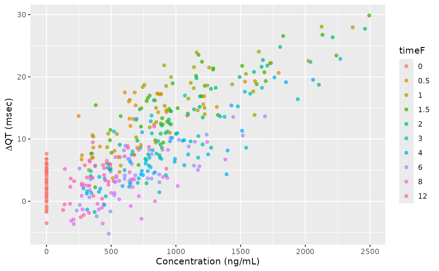

Fitting the model

Algebraic models with both a factor and a continuous covariate on the same parameter can be hard for focei’s gradient calculation when there are many factor levels. A robust two-stage strategy is to fit the fixed effects with bobyqa (which is gradient-free and converges fast for this class of model) and then refine with focei using the bobyqa estimates as starts, which adds the random effect.

fitFE :=
  nlmixr(
    dQT ~ b,                                       # fixed effects only
    data  = cqtData,
    start = list(
      b     = c(0, 3, 5, 6, 5, 2, 0, -1, -2, -3, 0.01),
      addSd = 3
    ),
    param = list(b ~ timeF + conc),
    est   = "bobyqa"
  )
#> ℹ loading fit from nlmixrFormula-fitFE.zip
#> ℹ loading fit from fitFE.R
#> ℹ parameter labels from comments are typically ignored in non-interactive mode
#> ℹ Need to run with the source intact to parse comments
#> ℹ removing unzipped fit files

fitFE

$$\begin{align*} {b} & = {b.timeF.0}+{b.timeF.0.5} {\times} \left({timeF}{\equiv}\text{"0.5"}\right)+{b.timeF.1} {\times} \left({timeF}{\equiv}\text{"1"}\right)+{b.timeF.1.5} {\times} \left({timeF}{\equiv}\text{"1.5"}\right)+{b.timeF.2} {\times} \left({timeF}{\equiv}\text{"2"}\right)+{b.timeF.3} {\times} \left({timeF}{\equiv}\text{"3"}\right)+{b.timeF.4} {\times} \left({timeF}{\equiv}\text{"4"}\right)+{b.timeF.6} {\times} \left({timeF}{\equiv}\text{"6"}\right)+{b.timeF.8} {\times} \left({timeF}{\equiv}\text{"8"}\right)+{b.timeF.12} {\times} \left({timeF}{\equiv}\text{"12"}\right)+{cov\_conc\_b} {\times} {conc} \\ {value} & = {b} \\ {value} & \sim add({addSd}) \end{align*}$$

# Carry the bobyqa estimates forward as starts for focei + random effects
feEst <- setNames(fitFE$iniDf$est, fitFE$iniDf$name)

fitRE :=
  nlmixr(
    dQT ~ b + bRe ~ (bRe|id),
    data  = cqtData,
    start = list(
      b     = c(feEst[1:10], feEst[["cov_conc_b"]]),
      addSd = feEst[["addSd"]]
    ),
    param = list(b ~ timeF + conc),
    est   = "focei"
  )
#> ℹ loading fit from nlmixrFormula-fitRE.zip
#> ℹ loading fit from fitRE.R
#> ℹ parameter labels from comments are typically ignored in non-interactive mode
#> ℹ Need to run with the source intact to parse comments
#> ℹ removing unzipped fit files

fitRE

$$\begin{align*} {b} & = {b.timeF.0}+{b.timeF.0.5} {\times} \left({timeF}{\equiv}\text{"0.5"}\right)+{b.timeF.1} {\times} \left({timeF}{\equiv}\text{"1"}\right)+{b.timeF.1.5} {\times} \left({timeF}{\equiv}\text{"1.5"}\right)+{b.timeF.2} {\times} \left({timeF}{\equiv}\text{"2"}\right)+{b.timeF.3} {\times} \left({timeF}{\equiv}\text{"3"}\right)+{b.timeF.4} {\times} \left({timeF}{\equiv}\text{"4"}\right)+{b.timeF.6} {\times} \left({timeF}{\equiv}\text{"6"}\right)+{b.timeF.8} {\times} \left({timeF}{\equiv}\text{"8"}\right)+{b.timeF.12} {\times} \left({timeF}{\equiv}\text{"12"}\right)+{cov\_conc\_b} {\times} {conc} \\ {value} & = {b}+{bRe} \\ {value} & \sim add({addSd}) \end{align*}$$

The recovered cov_conc_b estimates the slope of concentration on $\Delta QT$. Multiplying by the population $C_{max}$ (about 1000 ng/mL) gives the projected $\Delta QT$ at $C_{max}$ – typically within ~1 msec of the simulated 10 msec.

Defining the model equation (the formula)

The model formula has 3 parts: the dependent variable, the equation predicting the dependent variable, and the optional random effects. A full equation looks like the below:

dv~predictors~randomEffects

Any model part may have any parameter name (for example, the dependent variable does not have to be named dv).

Dependent variable

The dependent variable may be any column in the data. It must only be the column name and no additional modifiers. For example, log(param) is not allowed.

Predictors

Predictors may be any algebraic equation. In general, there are no restrictions to the way that the equation may be written.

Random effects

Random effects are not required for a model; fixed-effect-only models are possible. When present, fixed and random effects must have different names.

Random effects are written as a parameter a pipe (|) and its grouping value. From the quick start example above, the parameter is bRe and the grouping value is id, so it is written bRe|id.

For multiple parameters, they must be setup separately. For example, to have mRe and bRe both grouped by id, it would be defined as ~(mRe|id)+(bRe|id).

Only one grouping variable is supported per model. Multiple grouping variables (for inter-occasion variability, for example) are not yet supported.

Per-parameter covariate models (param)

The param argument adds a covariate model to one or more parameters. It accepts a formula or a list of formulas, each of the form <parameter> ~ <covariate columns>. The right-hand side names one or more columns from data:

• A factor column produces one fixed effect per level. The first level is the baseline; subsequent levels are estimated as differences from the baseline.
• A numeric column produces a slope. With only the continuous covariate, two parameters are introduced – pop.<parameter> (intercept) and cov_<column>_<parameter> (slope).
• Multiple covariates can be combined on the same parameter with +: b ~ z + w combines factor z and continuous w. When a factor is present, the factor supplies the baseline so pop.b is not introduced.

When mixing factor and continuous covariates on the same parameter, start[[<parameter>]] must explicitly list one value per factor level followed by one slope per continuous covariate (in the order they appear in param).

paramLink (link function per parameter)

By default the assembled linear combination is the parameter itself (b <- <linear combination>). Set paramLink = c(b = "log") to wrap the combination in exp(), so the parameter is strictly positive on its natural scale.

Providing the Starting estimates for the model

Fixed effects

Fixed effects are defined by the start argument. The start argument may either be a named vector or a named list. If fixed effects only have a single starting value, then the two methods are equivalent. c(m=3, b=5) is the same as list(m=3, b=5). If one of the fixed effects is defined by a factor variable (more on that later), the list may have multiple starting values such as list(m=3, b=c(5, 10)).

For continuous covariates passed via param, start[[<parameter>]] may be a single intercept value (the slope defaults to 0) or c(intercept, slope).

Random effects

Random effect starting values are currently fixed at 1 without the ability to modify it.

Residual error models

The default residual error model is ~ add(addSd) (additive standard deviation addSd). More complex specifications are supported as long as every sigma parameter in the residual formula appears in start. For example:

nlmixr(
  y~m*x + b ~ (bRe|id),
  start = list(m=3, b=5, addSd=1, propSd=0.1),
  residualModel = ~ add(addSd) + prop(propSd),
  data = dSimNlme,
  est = "focei"
)