Simulate New dosing from NONMEM model

This page shows a simple work-flow for directly simulating a different dosing paradigm than what was modeled.

Step 1: Import the model

library(nonmem2rx)
library(rxode2)

library(nonmem2rx)

# First we need the location of the nonmem control stream Since we are running an example, we will use one of the built-in examples in `nonmem2rx`
ctlFile <- system.file("mods/cpt/runODE032.ctl", package="nonmem2rx")
# You can use a control stream or other file. With the development
# version of `babelmixr2`, you can simply point to the listing file

mod <- nonmem2rx(ctlFile, lst=".res", save=FALSE, determineError=FALSE)
#> ℹ getting information from  '/home/runner/work/_temp/Library/nonmem2rx/mods/cpt/runODE032.ctl'
#> ℹ reading in xml file
#> ℹ done
#> ℹ reading in phi file
#> ℹ done
#> ℹ reading in lst file
#> ℹ abbreviated list parsing
#> ℹ done
#> ℹ done
#> ℹ splitting control stream by records
#> ℹ done
#> ℹ Processing record $INPUT
#> ℹ Processing record $MODEL
#> ℹ Processing record $THETA
#> ℹ Processing record $OMEGA
#> ℹ Processing record $SIGMA
#> ℹ Processing record $PROBLEM
#> ℹ Processing record $DATA
#> ℹ Processing record $SUBROUTINES
#> ℹ Processing record $PK
#> ℹ Processing record $DES
#> ℹ Processing record $ERROR
#> ℹ Processing record $ESTIMATION
#> ℹ Ignore record $ESTIMATION
#> ℹ Processing record $COVARIANCE
#> ℹ Ignore record $COVARIANCE
#> ℹ Processing record $TABLE
#> ℹ change initial estimate of `theta1` to `1.37034036528946`
#> ℹ change initial estimate of `theta2` to `4.19814911033061`
#> ℹ change initial estimate of `theta3` to `1.38003493562413`
#> ℹ change initial estimate of `theta4` to `3.87657341967489`
#> ℹ change initial estimate of `theta5` to `0.196446108190896`
#> ℹ change initial estimate of `eta1` to `0.101251418415006`
#> ℹ change initial estimate of `eta2` to `0.0993872449483344`
#> ℹ change initial estimate of `eta3` to `0.101302674763154`
#> ℹ change initial estimate of `eta4` to `0.0730497519364148`
#> ℹ read in nonmem input data (for model validation): /home/runner/work/_temp/Library/nonmem2rx/mods/cpt/Bolus_2CPT.csv
#> ℹ ignoring lines that begin with a letter (IGNORE=@)'
#> ℹ applying names specified by $INPUT
#> ℹ subsetting accept/ignore filters code: .data[-which((.data$SD == 0)),]
#> ℹ done
#> ℹ read in nonmem IPRED data (for model validation): /home/runner/work/_temp/Library/nonmem2rx/mods/cpt/runODE032.csv
#> ℹ done
#> ℹ changing most variables to lower case
#> ℹ done
#> ℹ replace theta names
#> ℹ done
#> ℹ replace eta names
#> ℹ done (no labels)
#> ℹ renaming compartments
#> ℹ done
#> ℹ solving ipred problem
#> ℹ done
#> ℹ solving pred problem
#> ℹ done

Step 2: Look at a different dosing paradigm

Lets say that in this case instead of a single dose, we want to see what the concentration profile is with a single day of BID dosing. In this case is done by creating a quick event table:

ev <- et(amt=120000, ii=12, until=24) %>%
  et(list(c(0, 2), # add observations in windows
          c(4, 6),
          c(8, 12),
          c(14, 18),
          c(20, 26),
          c(28, 32),
          c(32, 36),
          c(36, 44))) %>%
  et(id=1:10)

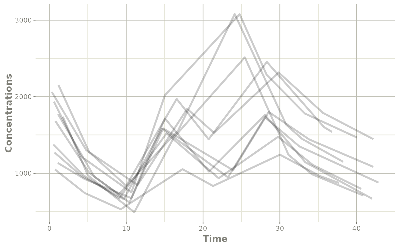
Step 3: solve using rxode2

In this step, we solve the model with the new event table for the 10 subjects:

s <- rxSolve(mod, ev)
#> ℹ using nocb interpolation like NONMEM, specify directly to change
#> ℹ using addlKeepsCov=TRUE like NONMEM, specify directly to change
#> ℹ using addlDropSs=TRUE like NONMEM, specify directly to change
#> ℹ using ssAtDoseTime=TRUE like NONMEM, specify directly to change
#> ℹ using safeZero=FALSE since NONMEM does not use protection by default
#> ℹ using ss2cancelAllPending=FALSE since NONMEM does not cancel pending doses with SS=2
#> ℹ using sigma from NONMEM
#> ℹ using NONMEM specified atol=1e-12
#> ℹ using NONMEM specified rtol=1e-06
#> ℹ using NONMEM specified ssAtol=1e-12

Note that since this is a nonmem2rx model, the default solving will match the tolerances and methods specified in your NONMEM model.

Step 4: exploring the simulation (by plotting)

This solved object acts the same as any other rxode2 solved object, so you can use the plot() function to see the individual profiles you simulated:

library(ggplot2)
plot(s, ipred) +
  ylab("Concentrations")