Plot a nlmixr2 data object

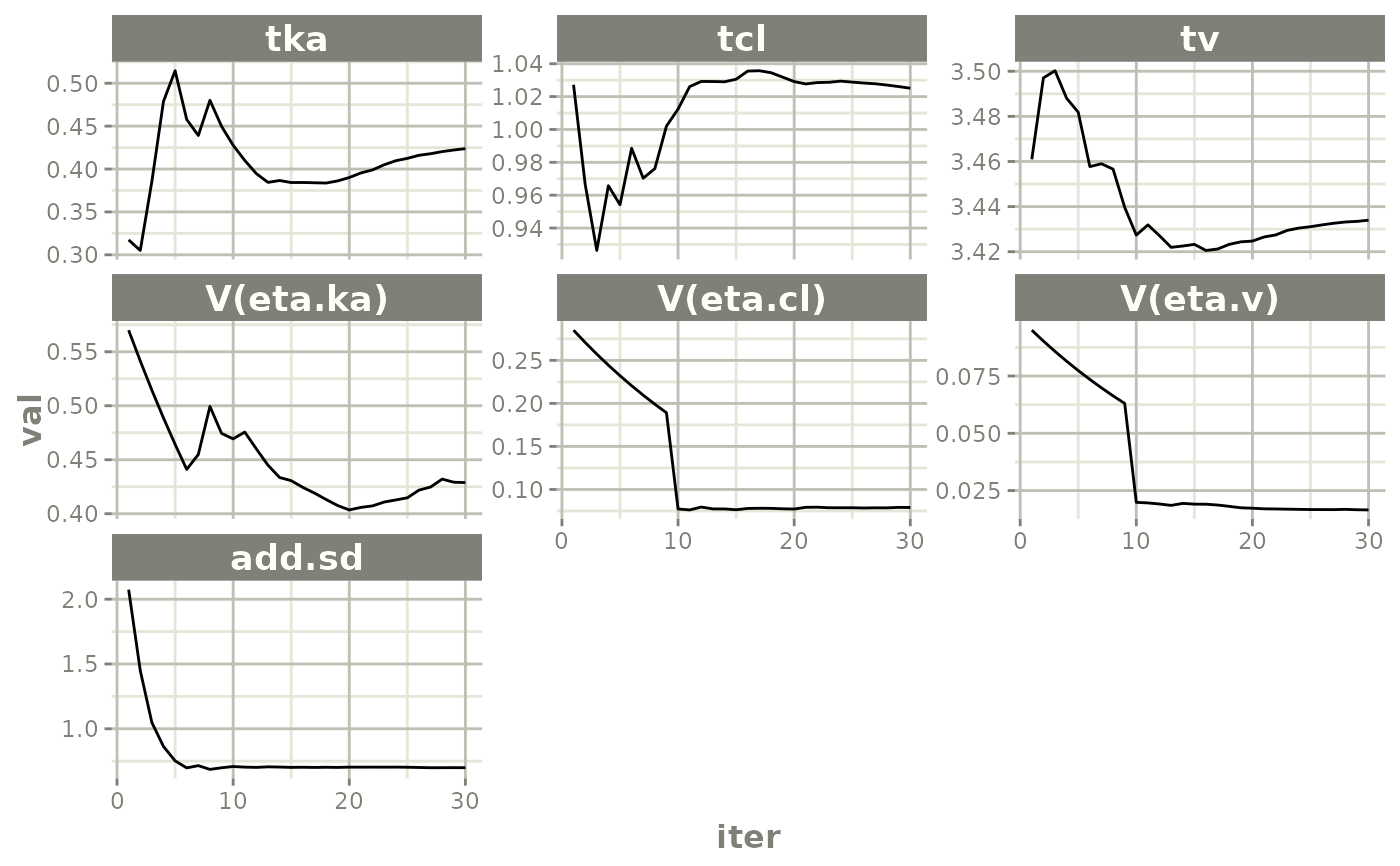
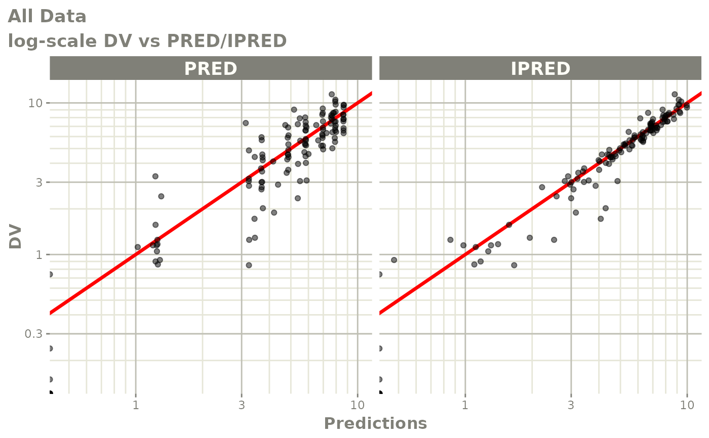
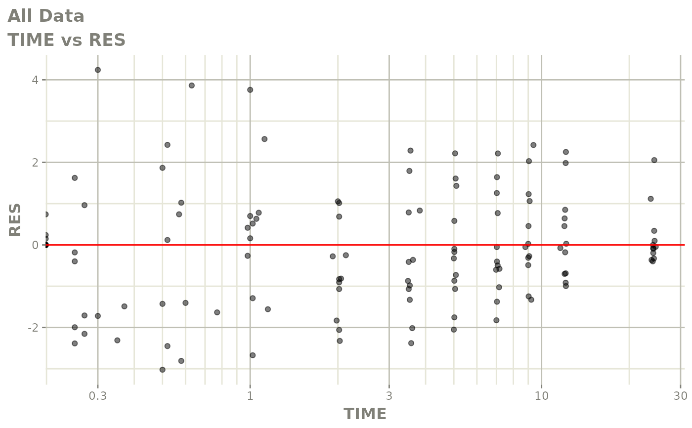
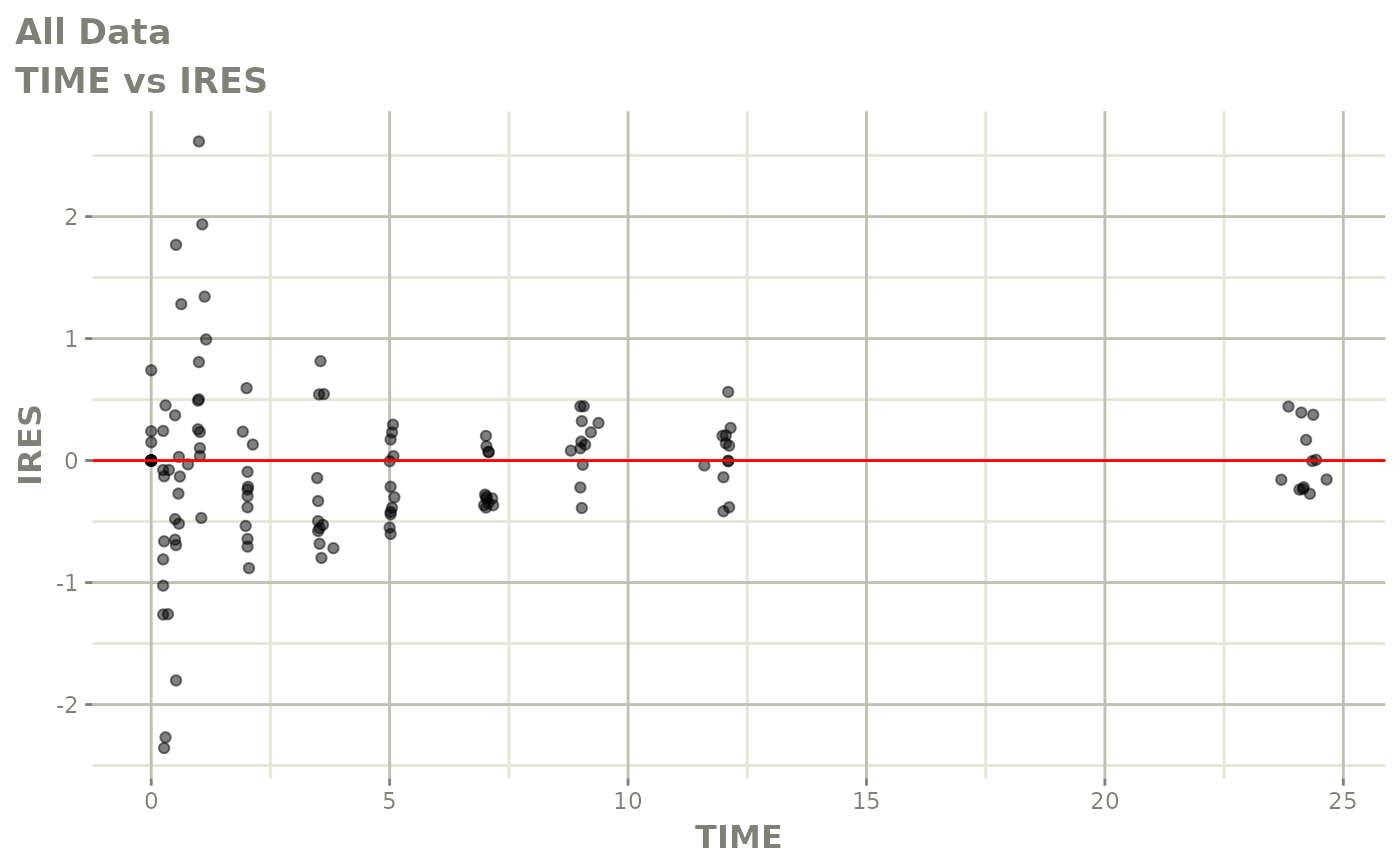
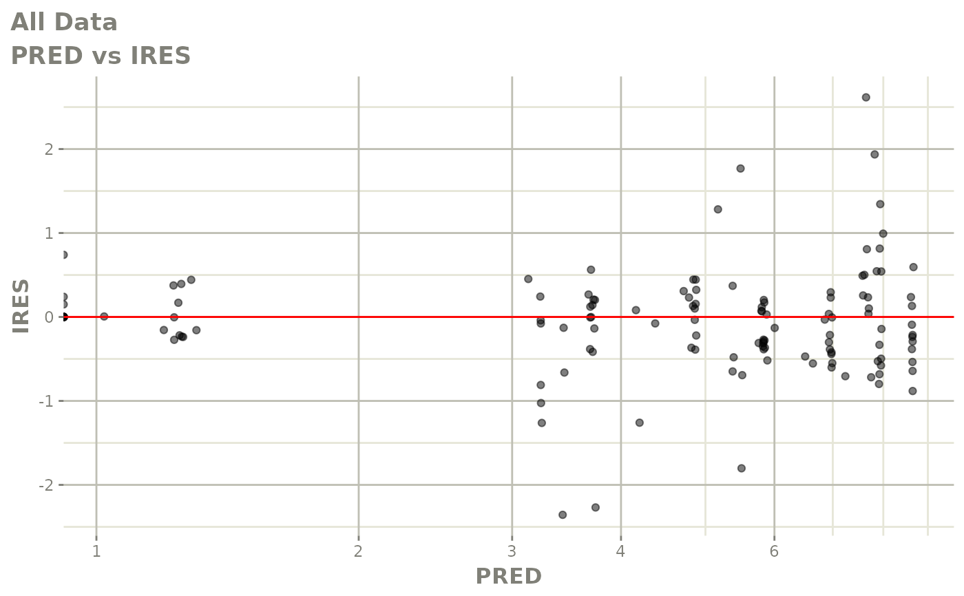
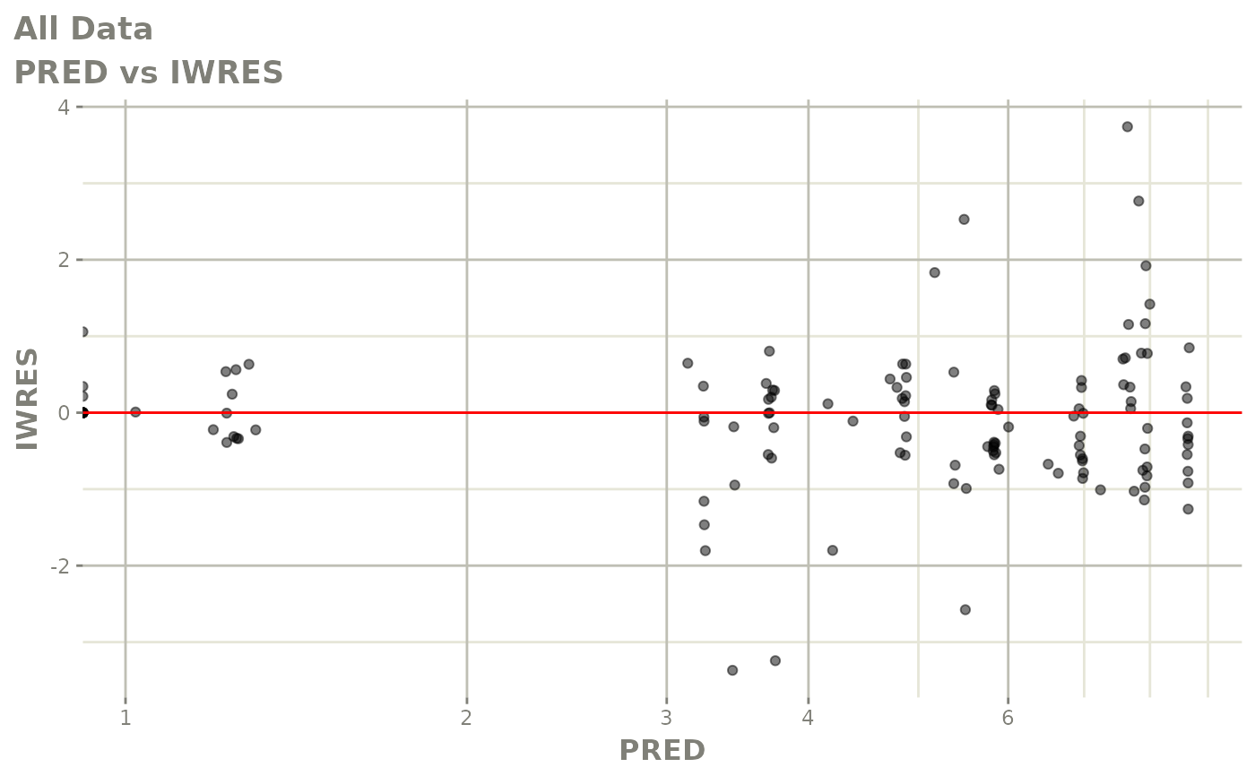
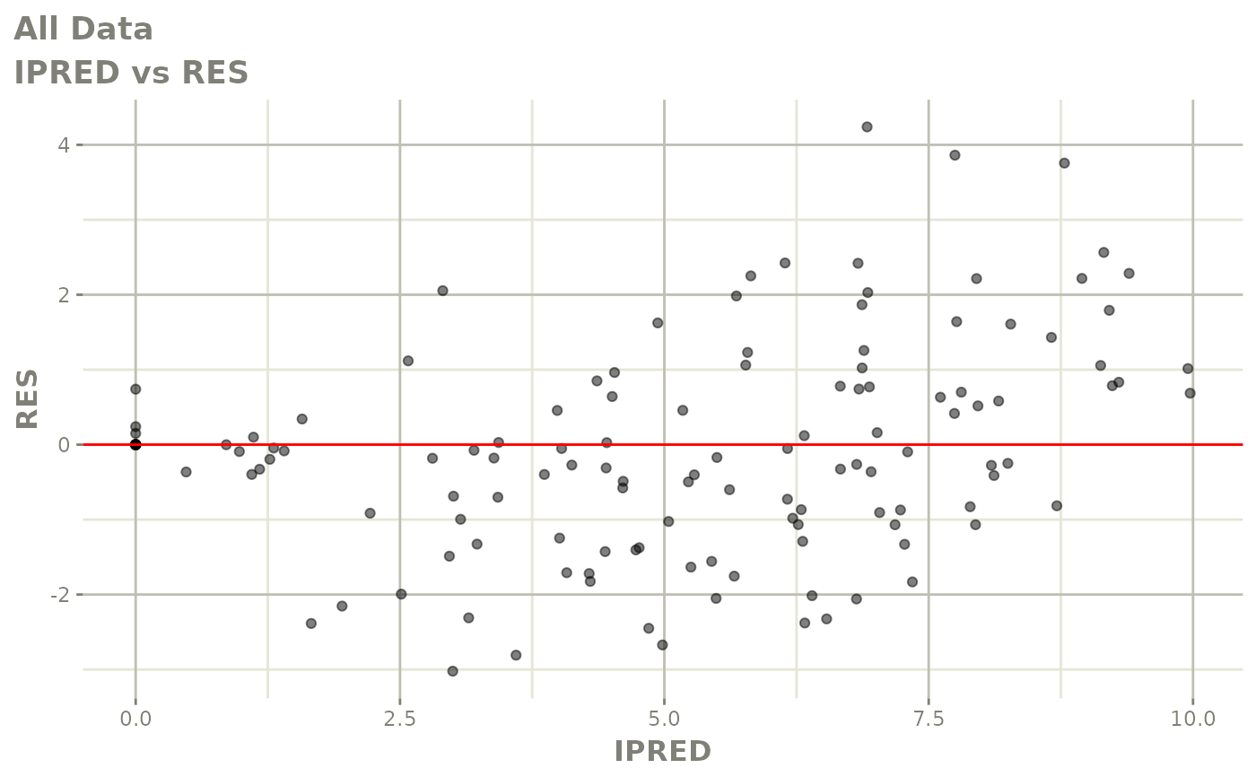
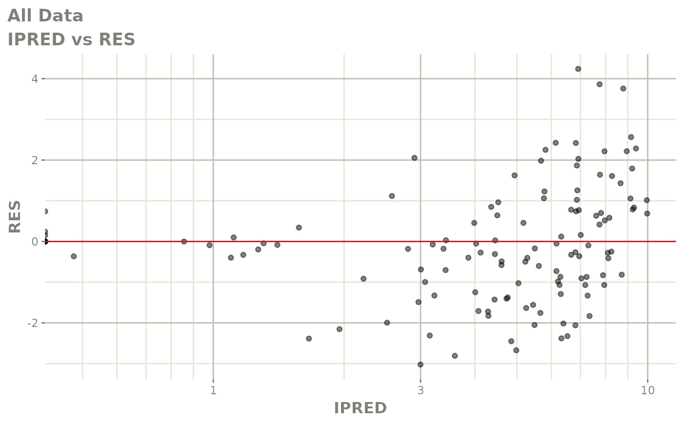
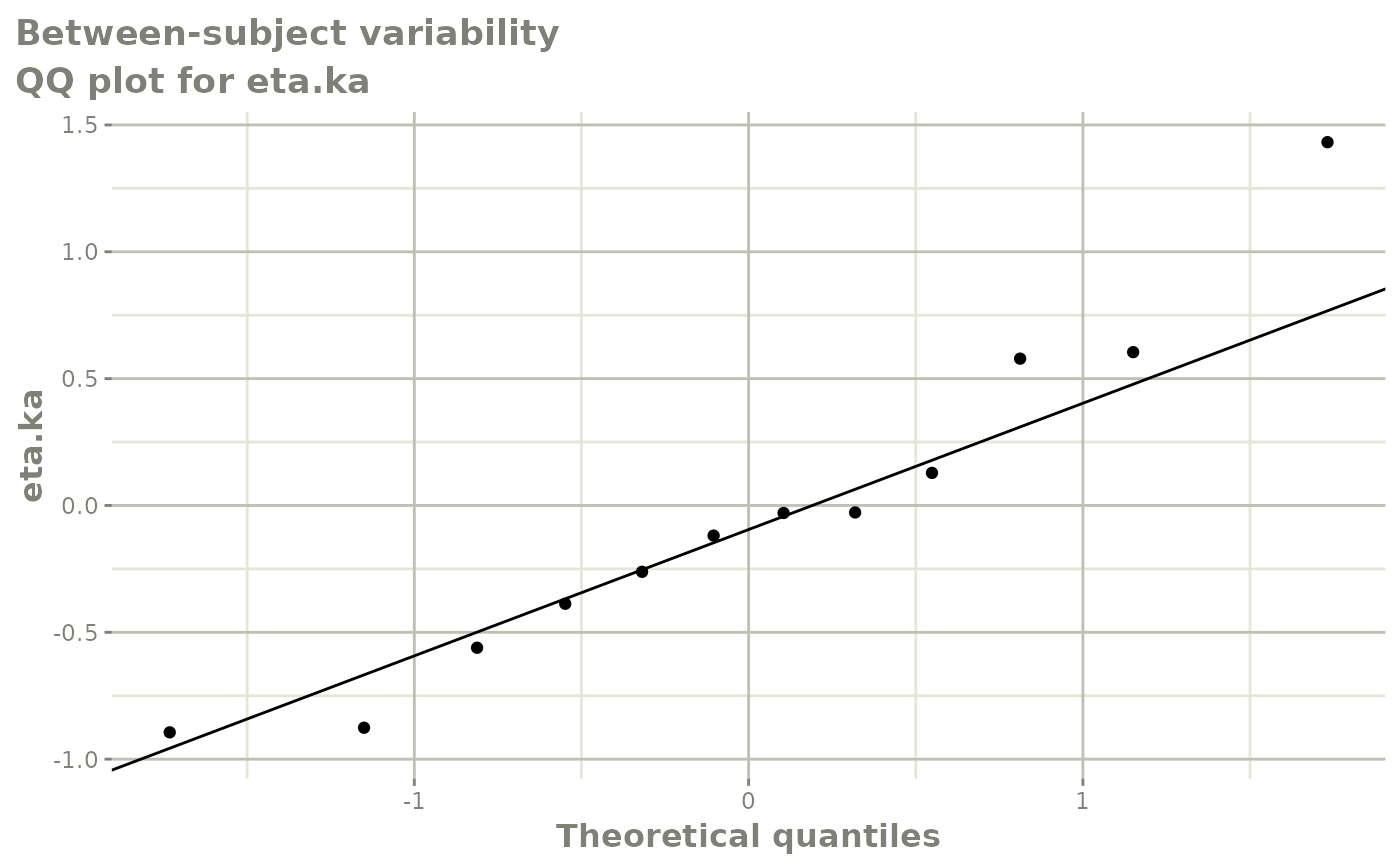
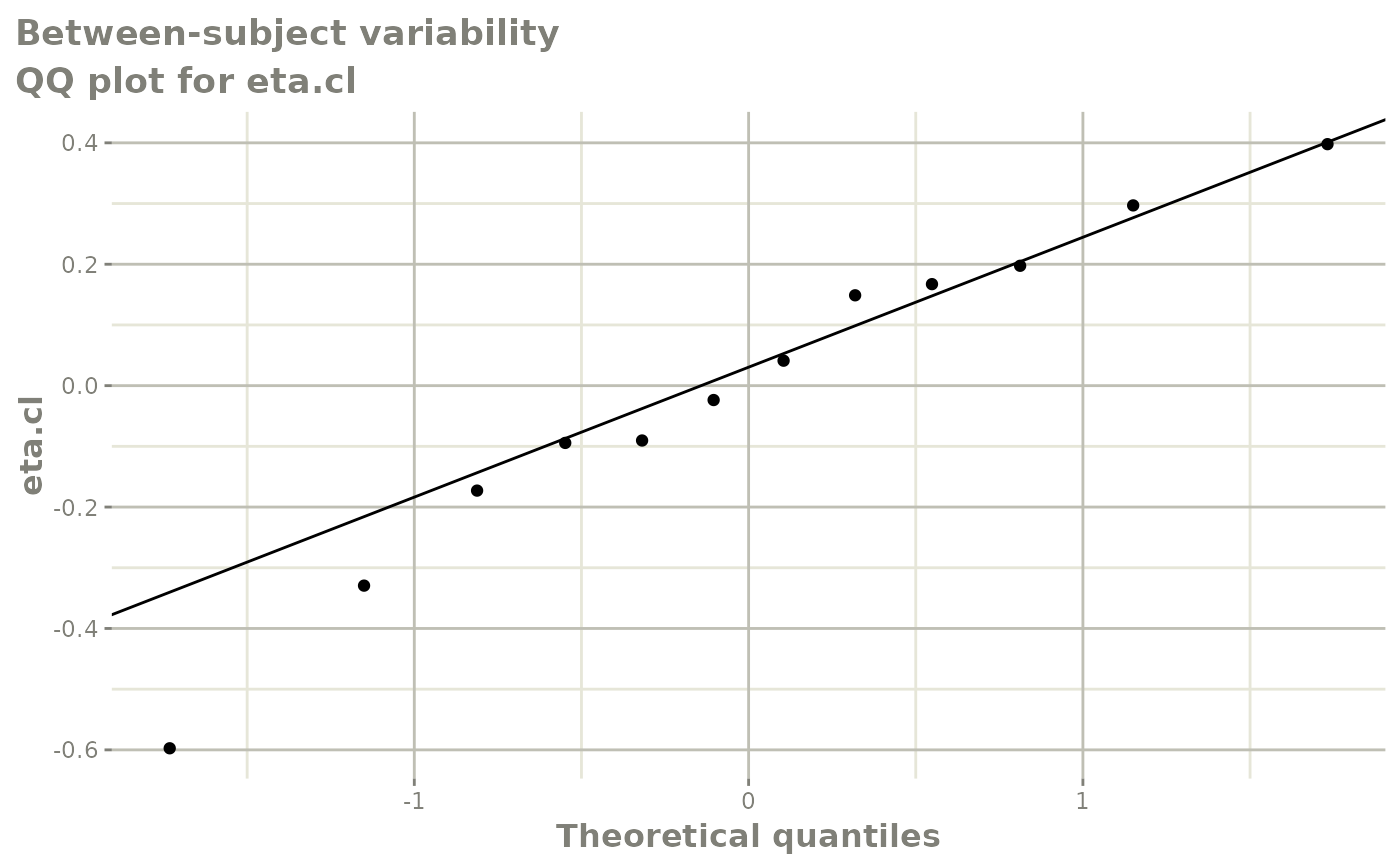
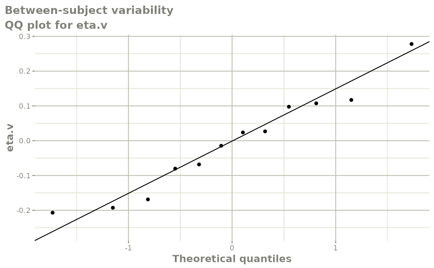
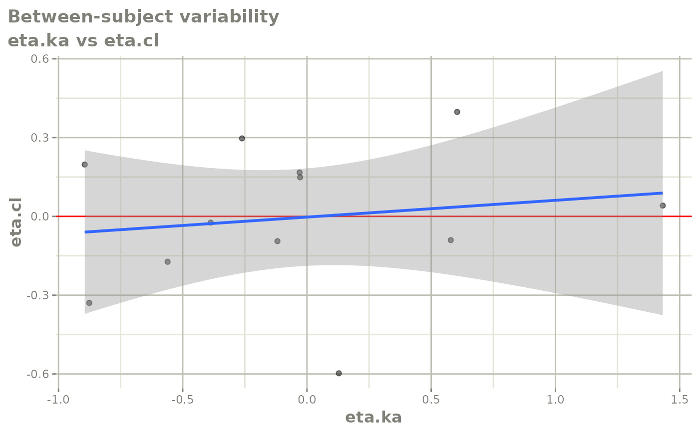
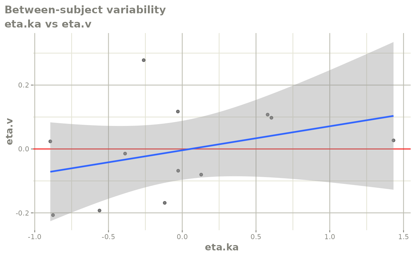
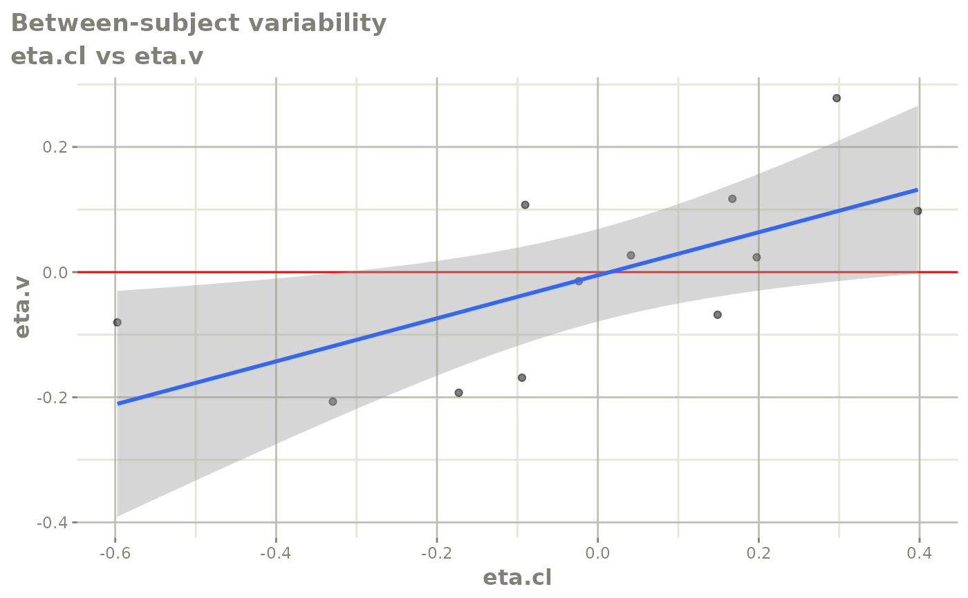
Plot some standard goodness of fit plots for the focei fitted object. When the model has between-subject variability (BSV), the returned collection also includes a nested "bsv" element (inside each data/compartment group) with QQ plots for each BSV parameter, BSV-BSV correlation plots (when more than one BSV parameter is present) and, when covariate is supplied, BSV-by-covariate plots.

Usage

# S3 method for class 'nlmixr2FitData'
plot(x, covariate = NULL, ...)

Arguments

x

a focei fit object

covariate

Optional character vector of covariate column names (from the model input data) to plot against each between-subject variability (BSV) parameter. Default NULL (no covariate plots). The first row per individual is used, so covariates are assumed time-invariant (a time-varying covariate is represented by its baseline value).

...

additional arguments (currently ignored)

Value

A named, nested ggtibble::gglist object (a list of ggplot2 objects with easier plotting of all of them at the same time)

Author

Wenping Wang & Matthew Fidler

Examples

# \donttest{
library(nlmixr2est)
one.compartment <- function() {
  ini({
    tka <- 0.45
    tcl <- 1
    tv <- 3.45
    eta.ka ~ 0.6
    eta.cl ~ 0.3
    eta.v ~ 0.1
    add.sd <- 0.7
  })
  model({
    ka <- exp(tka + eta.ka)
    cl <- exp(tcl + eta.cl)
    v <- exp(tv + eta.v)
    d/dt(depot) = -ka * depot
    d/dt(center) = ka * depot - cl / v * center
    cp = center / v
    cp ~ add(add.sd)
  })
}

## The fit is performed by the function nlmixr/nlmix2 specifying the model, data and estimate
fit <- nlmixr2(one.compartment, theo_sd,  est="saem", saemControl(print=0, nBurn = 10, nEm = 20))
#>  
#>  
#>  
#>  
#> ℹ parameter labels from comments are typically ignored in non-interactive mode
#> ℹ Need to run with the source intact to parse comments
#>  
#>  
#> → loading into symengine environment...
#> → pruning branches (`if`/`else`) of saem model...
#> ✔ done
#> → finding duplicate expressions in saem model...
#> → optimizing duplicate expressions in saem model...
#> ✔ done
#> ℹ calculate uninformed etas
#> ℹ done
#> Calculating covariance matrix
#> → loading into symengine environment...
#> → pruning branches (`if`/`else`) of saem model...
#> ✔ done
#> → finding duplicate expressions in saem predOnly model 0...
#> → finding duplicate expressions in saem predOnly model 1...
#> → optimizing duplicate expressions in saem predOnly model 1...
#> → finding duplicate expressions in saem predOnly model 2...
#> ✔ done
#>  
#>  
#> → Calculating residuals/tables
#> ✔ done
#> → compress origData in nlmixr2 object, save 6584
#> → compress parHistData in nlmixr2 object, save 2688
#> → compress phiM in nlmixr2 object, save 15016

# This shows many goodness of fit plots
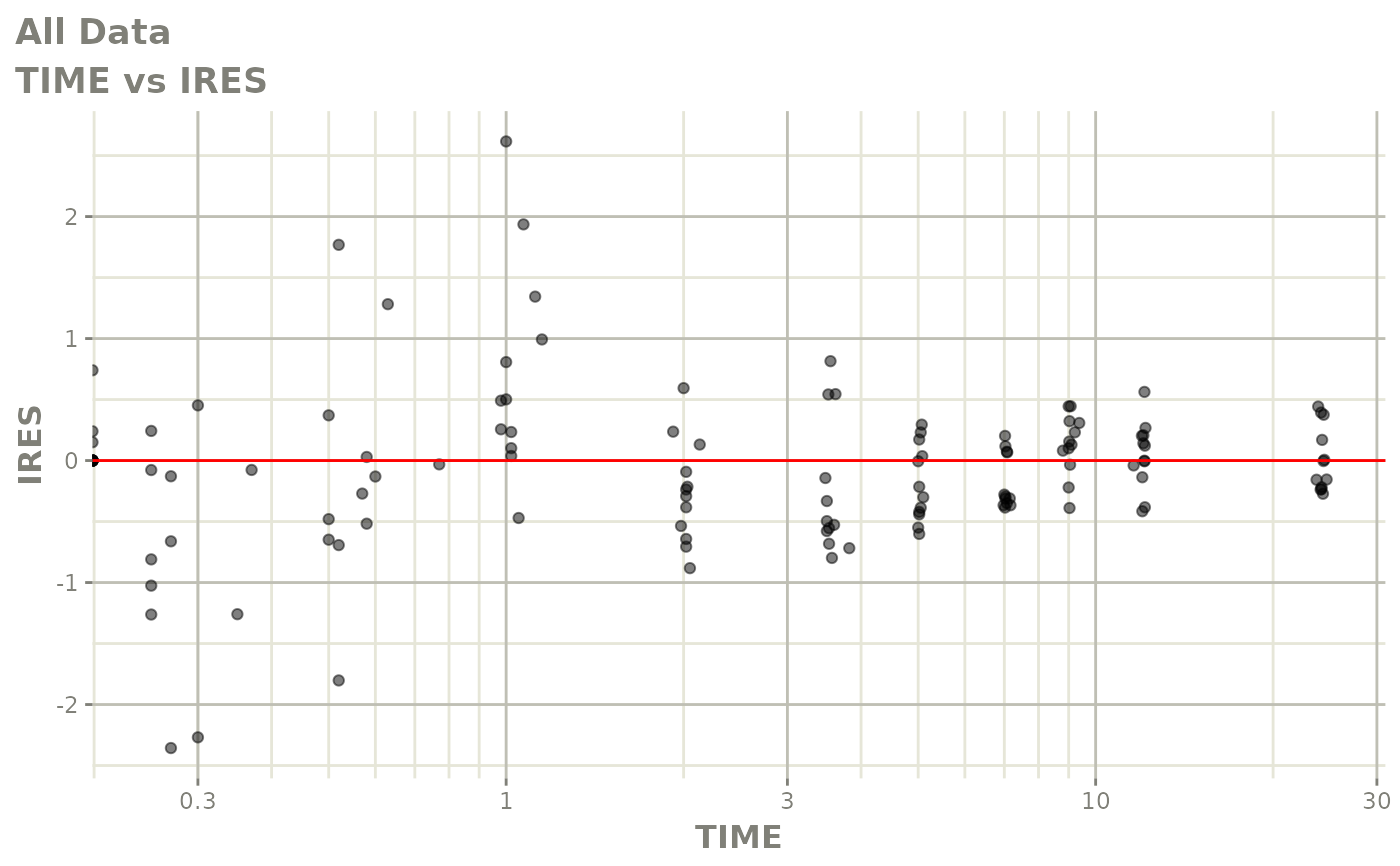
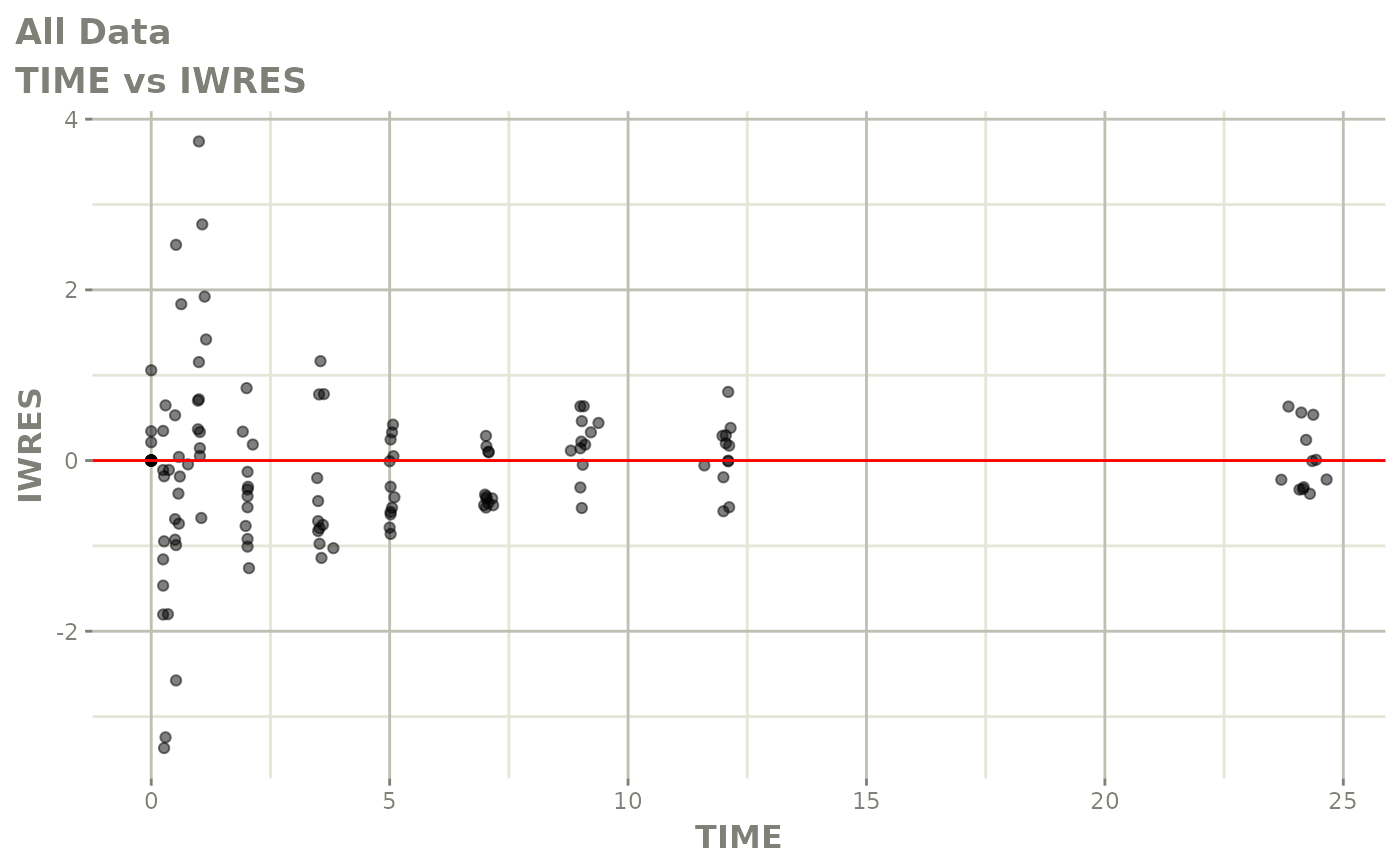
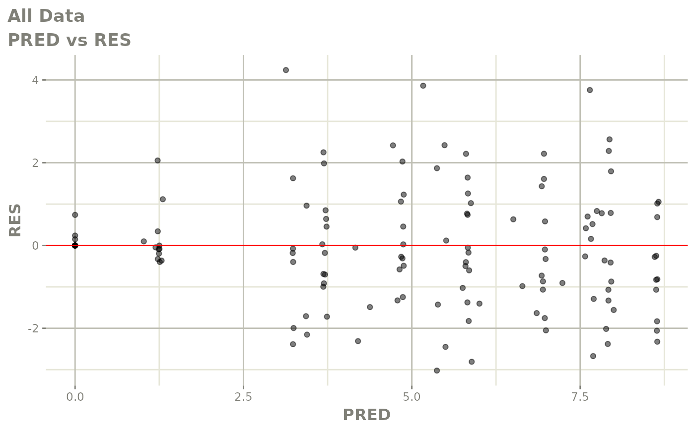
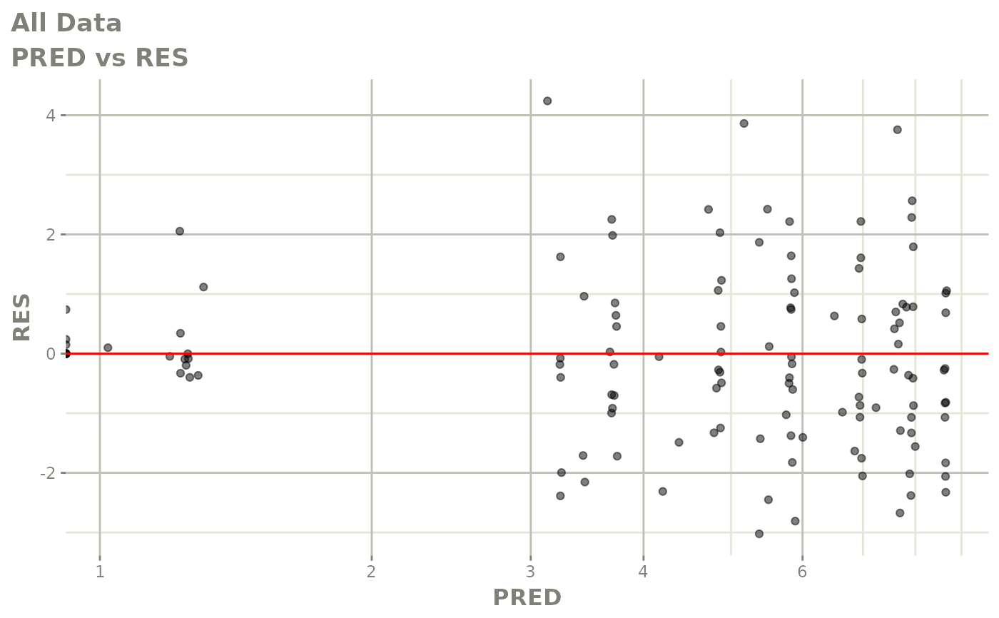
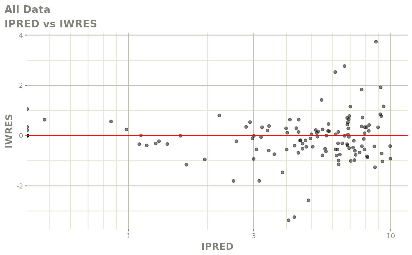
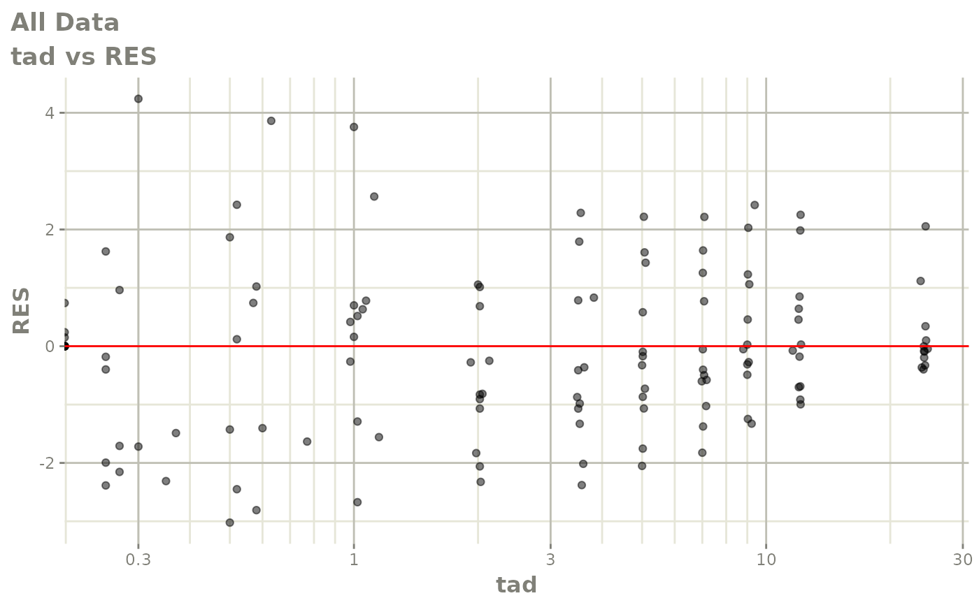
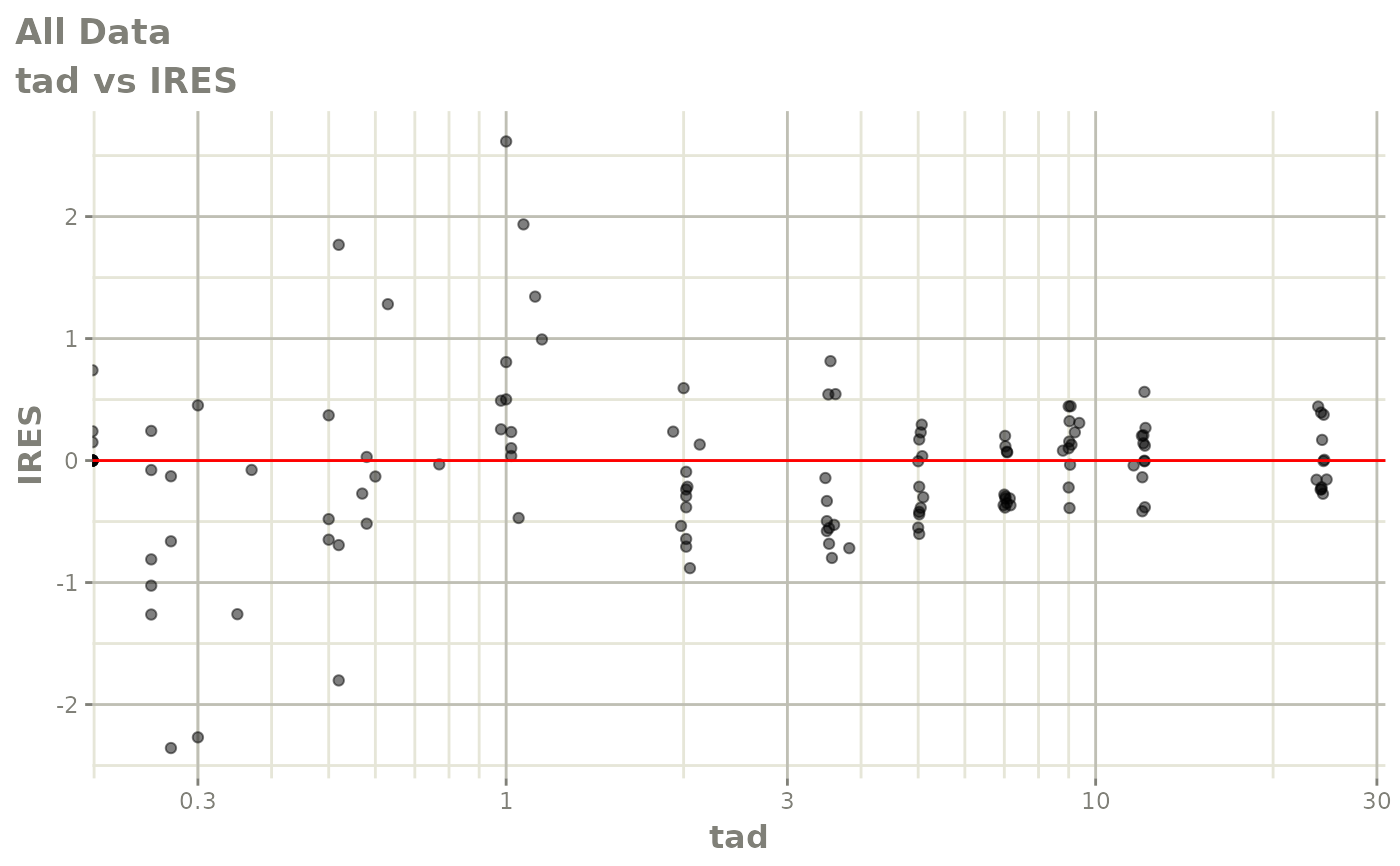
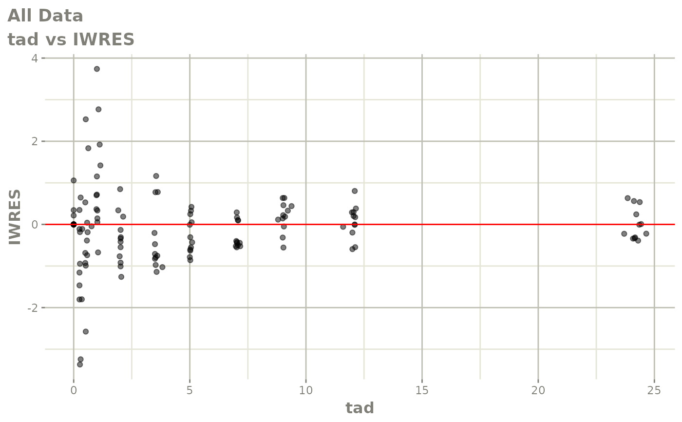
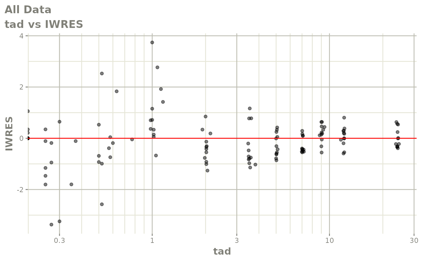
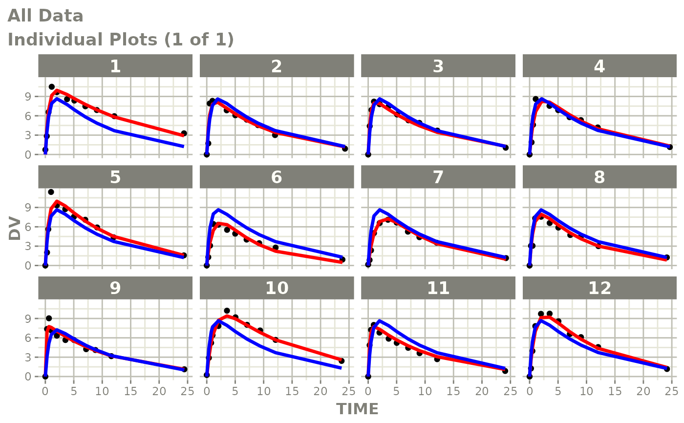
plot(fit)


#> Warning: log-10 transformation introduced infinite values.
#> Warning: log-10 transformation introduced infinite values.


#> Warning: log-10 transformation introduced infinite values.


#> Warning: log-10 transformation introduced infinite values.


#> Warning: log-10 transformation introduced infinite values.


#> Warning: log-10 transformation introduced infinite values.


#> Warning: log-10 transformation introduced infinite values.


#> Warning: log-10 transformation introduced infinite values.


#> Warning: log-10 transformation introduced infinite values.


#> Warning: log-10 transformation introduced infinite values.


#> Warning: log-10 transformation introduced infinite values.


#> Warning: log-10 transformation introduced infinite values.


#> Warning: log-10 transformation introduced infinite values.


#> Warning: log-10 transformation introduced infinite values.








# }